Chapter 16 - Dates and times
library(lubridate)
library(nycflights13)
16.2.4 Exercises
1. What happens if you parse a string that contains invalid dates?
You get an error message telling you the number of strings that failed to parse. In this instance, the error message is “1 failed to parse.” A vector is returned containing the strings of dates that parsed correctly with the invalid dates replaced with NA.
ymd(c("2010-10-10", "bananas"))## Warning: 1 failed to parse.## [1] "2010-10-10" NA2. What does the tzone argument to today() do? Why is it important?
The documentation states that the tzone argument in today() accepts a character vector specifying the time zone you would like to find the curent date of. It will default to the system time zone on your computer if left unspecified. This is important because, depending on the time zone, the date could be different. For example, the US west coast is 3 hours behind the US east coast. If it is 11PM on the west coast, the east coast is one day ahead. Below is the example provided in the documentation.
today()## [1] "2020-01-21"today("GMT")## [1] "2020-01-22"today() == today("GMT") # not always true## [1] FALSE3. Use the appropriate lubridate function to parse each of the following dates:
Based on the format of the string, the order of the month, year, and day parameters will determine which appropriate lubridate function should be used. For example, the first string, d1, is in month-day-year format, so we should use the lubridate function mdy. I apply the same principle to the other cases.
d1 <- "January 1, 2010"
d2 <- "2015-Mar-07"
d3 <- "06-Jun-2017"
d4 <- c("August 19 (2015)", "July 1 (2015)")
d5 <- "12/30/14" # Dec 30, 2014

mdy(d1)
## [1] "2010-01-01"ymd(d2)## [1] "2015-03-07"dmy(d3)## [1] "2017-06-06"mdy(d4)## [1] "2015-08-19" "2015-07-01"mdy(d5)## [1] "2014-12-30"16.3.4 Exercises
make_datetime_100 <- function(year, month, day, time) {
  make_datetime(year, month, day, time %/% 100, time %% 100)
}

flights_dt <- flights %>%
  filter(!is.na(dep_time), !is.na(arr_time)) %>%
  mutate(
    dep_time = make_datetime_100(year, month, day, dep_time),
    arr_time = make_datetime_100(year, month, day, arr_time),
    sched_dep_time = make_datetime_100(year, month, day, sched_dep_time),
    sched_arr_time = make_datetime_100(year, month, day, sched_arr_time)
  ) %>%
  select(origin, dest, ends_with("delay"), ends_with("time"))

flights_dt
## # A tibble: 328,063 x 9
## origin dest dep_delay arr_delay dep_time sched_dep_time
## <chr> <chr> <dbl> <dbl> <dttm> <dttm>
## 1 EWR IAH 2 11 2013-01-01 05:17:00 2013-01-01 05:15:00
## 2 LGA IAH 4 20 2013-01-01 05:33:00 2013-01-01 05:29:00
## 3 JFK MIA 2 33 2013-01-01 05:42:00 2013-01-01 05:40:00
## 4 JFK BQN -1 -18 2013-01-01 05:44:00 2013-01-01 05:45:00
## 5 LGA ATL -6 -25 2013-01-01 05:54:00 2013-01-01 06:00:00
## 6 EWR ORD -4 12 2013-01-01 05:54:00 2013-01-01 05:58:00
## 7 EWR FLL -5 19 2013-01-01 05:55:00 2013-01-01 06:00:00
## 8 LGA IAD -3 -14 2013-01-01 05:57:00 2013-01-01 06:00:00
## 9 JFK MCO -3 -8 2013-01-01 05:57:00 2013-01-01 06:00:00
## 10 LGA ORD -2 8 2013-01-01 05:58:00 2013-01-01 06:00:00
## # … with 328,053 more rows, and 3 more variables: arr_time <dttm>,
## # sched_arr_time <dttm>, air_time <dbl>1. How does the distribution of flight times within a day change over the course of the year?
Within a day, we want to observe how the flight times differ. This means we should look at how flight times differ by the hour (ie how many flights are taking off at every hour of the day). Now, we want to see how this behavior changes over the course of the year (ie how does this graph look like when plotted monthly)? We observe that the distribution of flights within a day does not significantly change over the course of the year. The same trend is followed in which there is a peak of flights around 8am, a dip in flights from 10am-12pm, and then a slow drop off in number of flights past 7pm.
# flights per hour for the entire year
flights_dt %>%
  mutate(hour = hour(dep_time)) %>%
  group_by(hour)%>%
  summarize(numflights_per_hour = n())%>%
  ggplot(aes(x = hour, y = numflights_per_hour)) +
    geom_line()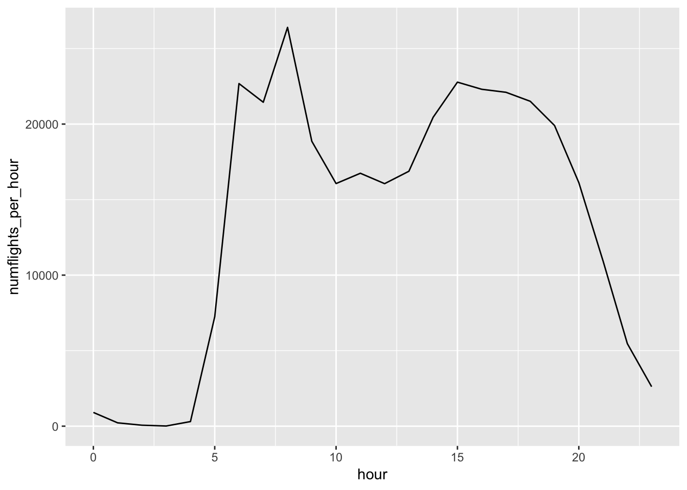
# split the above graph into months

flights_dt %>%
  mutate(hour = hour(dep_time),
         month = as.factor(month(dep_time))) %>%
  group_by(month,hour)%>%
  summarize(numflights_per_hour = n())%>%
  ggplot(aes(x = hour, y = numflights_per_hour)) +
    geom_line(aes(color = month))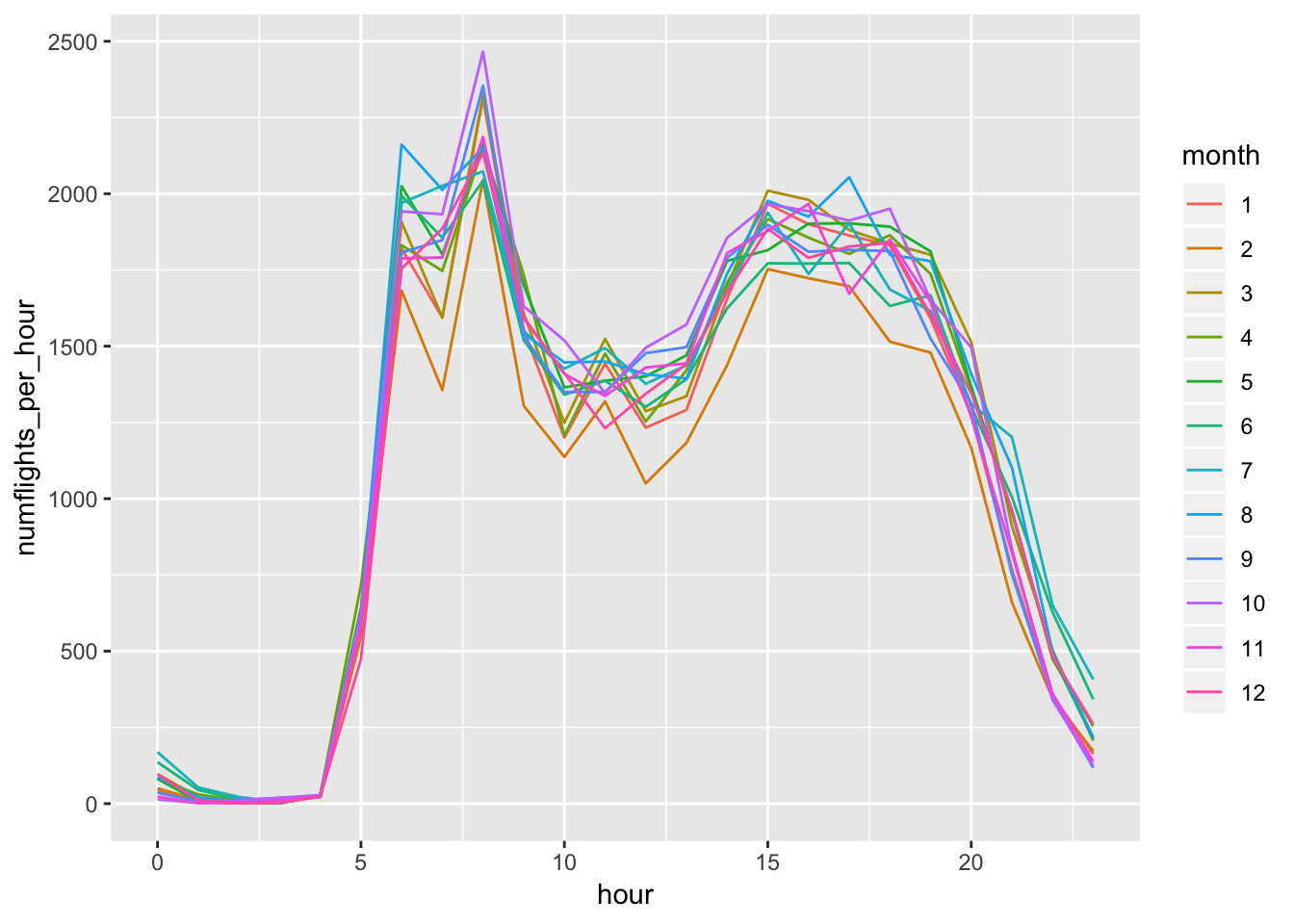
2. Compare dep_time, sched_dep_time and dep_delay. Are they consistent? Explain your findings.
First calculate our own version of dep_time by adding sched_dep_time and dep_delay together, then compare the result to the provided dep_time in the table. When filtering for values in dep_time that do not match the calculated version, we find 1205 discrepancies out of the 328,063 observations. For the most part, they are consistent, but we should find out why the 1205 inconsistencies exist.
flights_dt %>%
  mutate ( calculated_dep_time = sched_dep_time + dep_delay*60) %>%
  select (calculated_dep_time, sched_dep_time, dep_delay, dep_time) %>%
  filter ( calculated_dep_time != dep_time) %>%
  count()
## # A tibble: 1 x 1
## n
## <int>
## 1 12053. Compare air_time with the duration between the departure and arrival. Explain your findings. (Hint: consider the location of the airport.)
Theoretically, the duration should match the difference between the arrival time and hte departure time, after accounting for time zone differences between airport locations. If the time zone difference is not accounted for, the air_time will not match the simple difference. This seems to be the case, because 327,150 of the 328,063 observations in the dataset have a reported air_time that does not match the difference between the arrival and departure times.
flights_dt %>%
  mutate ( calculated_air_time = arr_time - dep_time) %>%
  select (calculated_air_time, air_time, arr_time, dep_time) %>%
  filter (calculated_air_time != air_time)
## # A tibble: 327,150 x 4
## calculated_air_time air_time arr_time dep_time
## <time> <dbl> <dttm> <dttm>
## 1 193 mins 227 2013-01-01 08:30:00 2013-01-01 05:17:00
## 2 197 mins 227 2013-01-01 08:50:00 2013-01-01 05:33:00
## 3 221 mins 160 2013-01-01 09:23:00 2013-01-01 05:42:00
## 4 260 mins 183 2013-01-01 10:04:00 2013-01-01 05:44:00
## 5 138 mins 116 2013-01-01 08:12:00 2013-01-01 05:54:00
## 6 106 mins 150 2013-01-01 07:40:00 2013-01-01 05:54:00
## 7 198 mins 158 2013-01-01 09:13:00 2013-01-01 05:55:00
## 8 72 mins 53 2013-01-01 07:09:00 2013-01-01 05:57:00
## 9 161 mins 140 2013-01-01 08:38:00 2013-01-01 05:57:00
## 10 115 mins 138 2013-01-01 07:53:00 2013-01-01 05:58:00
## # … with 327,140 more rows4. How does the average delay time change over the course of a day? Should you use dep_time or sched_dep_time? Why?
Use the hour() function to group observations based on hour, then group by this parameter. Use this to calculate the average dep_delay per hour over the year. Plot using geom_line(). This can also be achieved using date-time components function update(), although this would change the number of points connected on the graph. I’ve plotted both results using either dep_time or sched_dep_time. You should use sched_dep_time instead of dep_time since this will tell you which scheduled flights might have a higher chance of being delayed. We observe that flights scheduled later on during the day have higher chances of being delayed, with a peak around hour 20 (8pm). Organizing by dep_time will let you know what time of the day most of the flights are delayed, which will intuitively occur later than the scheduled time as the flights start backing up. We observe that this is indeed the case, in which the peak of the late flights for dep_time occurs after the peak for the sched_dep_time plot, in which the flights are now delayed past midnight.
flights_dt %>%
  mutate ( dep_hour = hour(sched_dep_time) )%>%
  group_by(dep_hour) %>%
  summarize(avg_delay_hour = mean(dep_delay, na.rm = T)) %>%
  ggplot(aes(dep_hour, avg_delay_hour)) +
    geom_line()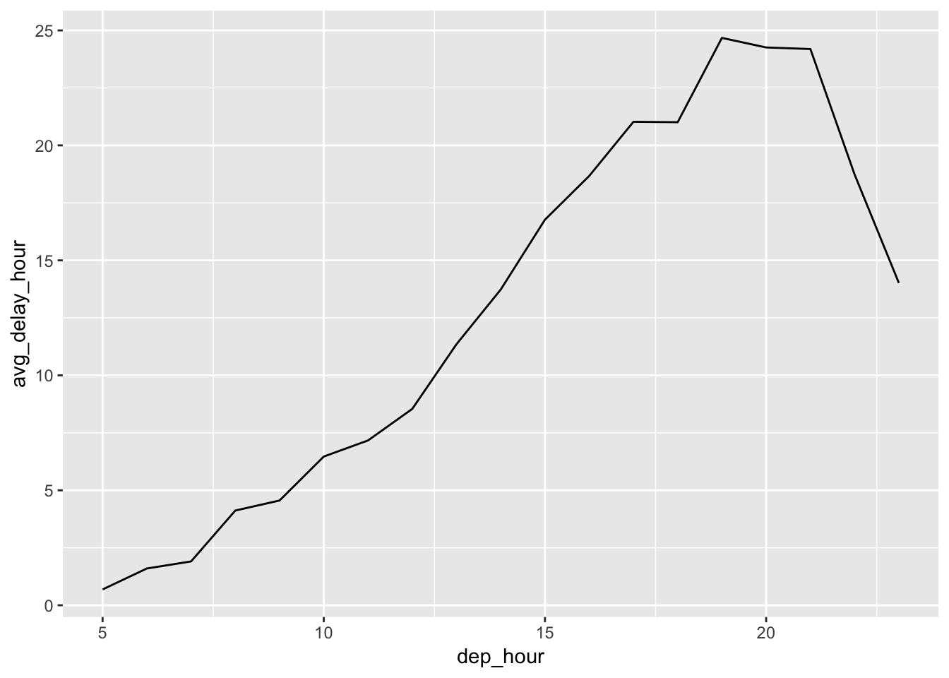
flights_dt %>%
  mutate ( dep_hour = hour(dep_time) )%>%
  group_by(dep_hour) %>%
  summarize(avg_delay_hour = mean(dep_delay, na.rm = T)) %>%
  ggplot(aes(dep_hour, avg_delay_hour)) +
    geom_line()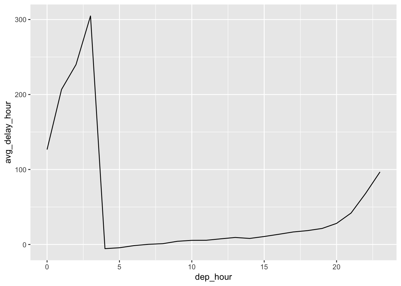
5. On what day of the week should you leave if you want to minimise the chance of a delay?
To find days of the week that have the lowest average delay, first assign a day to each observation using wday(). Then group by the day of the week, and use summarize() to find the average delay time on for each day of the week. We see that Saturday has the lowest average delay at 7.61, and on average the flights even arrive earlier than expected!
flights_dt %>%
  mutate(wday = wday(sched_dep_time, label = TRUE)) %>%
  group_by(wday) %>%
  summarize ( avg_dep_delay_week = mean(dep_delay, na.rm = TRUE),
              avg_arr_delay_week = mean(arr_delay, na.rm = TRUE))
## # A tibble: 7 x 3
## wday avg_dep_delay_week avg_arr_delay_week
## <ord> <dbl> <dbl>
## 1 Sun 11.5 4.82
## 2 Mon 14.7 9.65
## 3 Tue 10.6 5.39
## 4 Wed 11.7 7.05
## 5 Thu 16.1 11.7
## 6 Fri 14.7 9.07
## 7 Sat 7.62 -1.456. What makes the distribution of diamonds\(carat and flights\)sched_dep_time similar?
Let’s first examine the distribution of each of these datasets, using histograms. Using just the default value for binwidth, there is no apparent similarity between the distribution of values between the two datasets upon initial observation. The carat values are skewed to the right, but the sched_dep_time is not. I suppose one could argue that there are more flights with an earlier sched_dep_time, and likewise there are more diamonds with a low carat value. However, if we bin the values using smaller binwidth, we observe “spikes” of values in both datasets. This “spike” phenomenon occurs at carat 1, 1.5, 2, etc. and around flight times near the hour. This is likely an example of human “bias” for flights leaving at “nice” departure times, as mentioned by Hadley.
ggplot (diamonds, aes(x = carat)) +
  geom_histogram()
## `stat_bin()` using `bins = 30`. Pick better value with `binwidth`.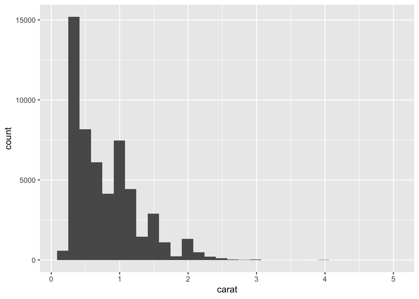
ggplot (flights, aes(x = sched_dep_time)) +
  geom_histogram()
## `stat_bin()` using `bins = 30`. Pick better value with `binwidth`.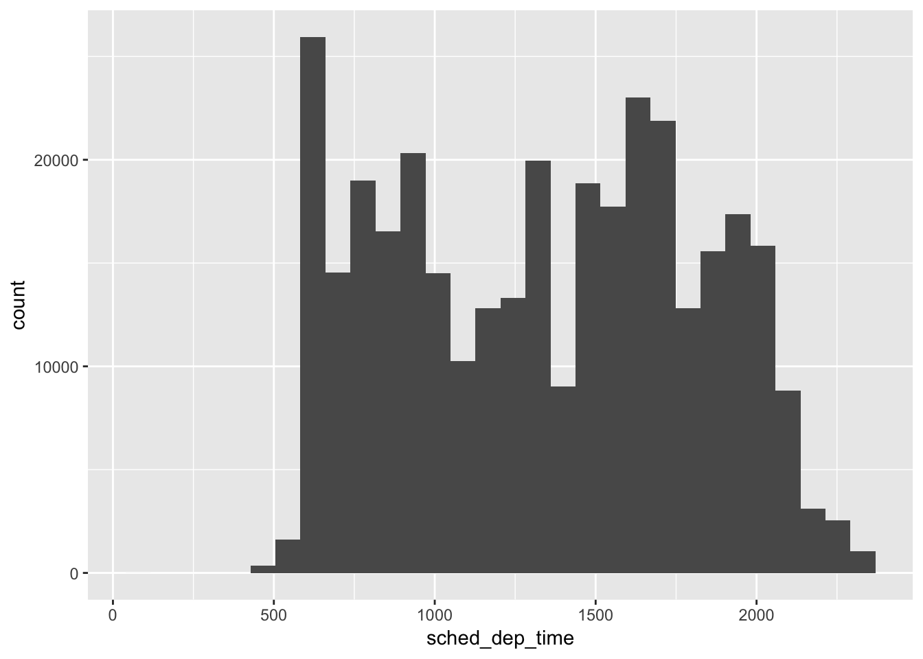
ggplot (diamonds, aes(x = carat)) +
  geom_freqpoly(binwidth = 0.1)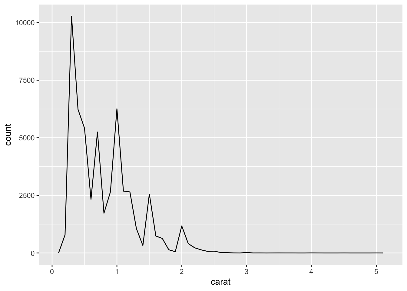
ggplot (flights, aes(x = sched_dep_time)) +
  geom_freqpoly(binwidth = 10)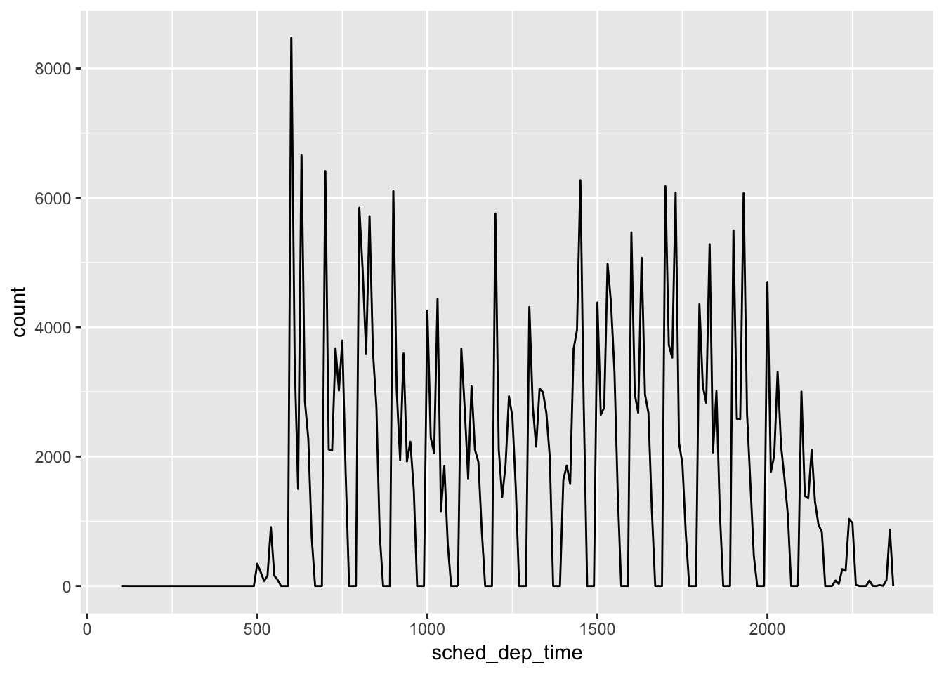
7. Confirm my hypothesis that the early departures of flights in minutes 20-30 and 50-60 are caused by scheduled flights that leave early. Hint: create a binary variable that tells you whether or not a flight was delayed.
To test this hypothesis, we need to see whether the total number of flights that departed early was increased during minutes 20-30 and 50-60. If this is true, then his hypothesis is supported. If this is not true, then maybe other factors are contributing more significantly to the lower flight delays during these time slots. To figure this out, we first use mutate() and ifelse() to assign whether or not a flight left early using TRUE or FALSE. Then, grouping by minute, we can count the number of flights that left early using sum(), and plot this value using ggplot(). We observe that there are indeed more flights leaving early during the 20-30 and 50-60 time slots (the graph looks like and inverted plot of the avg_delay by minute graph).
flights_dt %>%
  mutate(minute = minute(dep_time),
         early = ifelse(dep_delay>=0, FALSE, TRUE)) %>%
  group_by(minute) %>%
  summarise(
    avg_delay = mean(arr_delay, na.rm = TRUE),
    num_flights_early = sum(early),
    n = n()) %>%
  ggplot(aes(minute, num_flights_early)) +
    geom_line()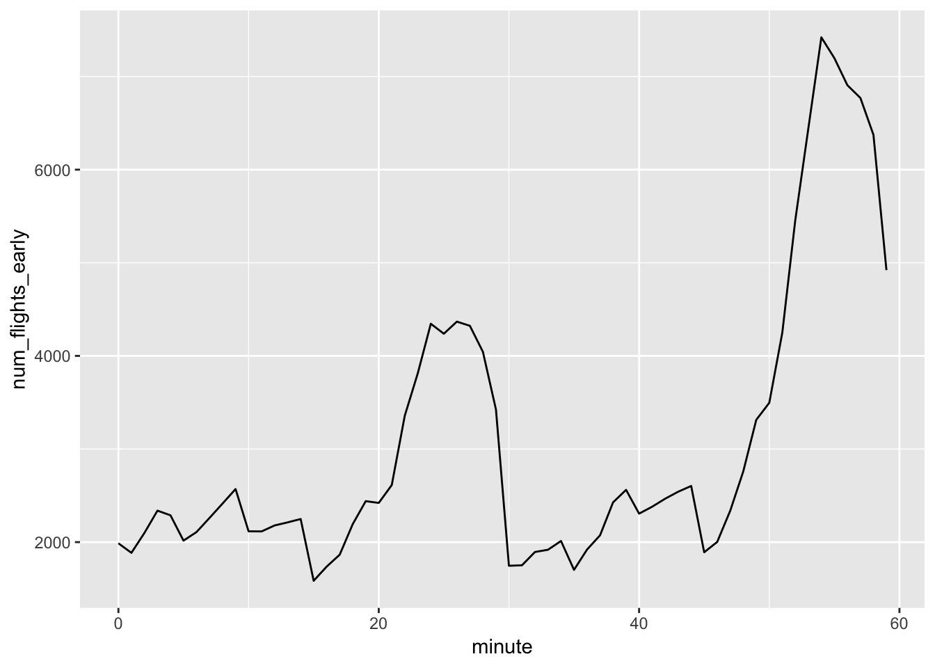
16.4.5 Exercises
1. Why is there months() but no dmonths()?
Durations must be standardized lengths of time. There is no dmonths() since months do not have a standard number of days. For example, February has a shorter number of days than January.
2. Explain days(overnight * 1) to someone who has just started learning R. How does it work?
The days() function converts the input into a datetime, for example, days(5) returns “5d 0H 0M 0S”. In this case, the input is overnight * 1. The variable overnight corresponds to the output of arr_time < dep_time, which is evaluated as a boolean (TRUE or FALSE). The multiplication with 1 will cause TRUE or FALSE to be converted to 1 or 0. Thus, days(overnight *1) will give you either 0 or 1 days in datetime form, which can then be added to arr_time.
# proof of concepts
days(5)
## [1] "5d 0H 0M 0S"TRUE*1## [1] 1FALSE*1## [1] 0days(1) + days (TRUE *1)## [1] "2d 0H 0M 0S"# Example from text using days (overnight * 1)
flights_dt <- flights_dt %>%
mutate(
overnight = arr_time < dep_time,
arr_time = arr_time + days(overnight * 1),
sched_arr_time = sched_arr_time + days(overnight * 1)
)3. Create a vector of dates giving the first day of every month in 2015. Create a vector of dates giving the first day of every month in the current year.
To do this, we can use ymd() to create a date for January 1, 2015. Then we can add this to a vector of months in order to generate a vector of 1st days for every month in that year. To do the first day of everymonth for the current year, we should write code that will work no matter what year you run it. To do this, we can use the today() function to get todays date, then extract the year from this date. This can be done two ways. You can either use floor_date(), which can round the date to the nearest year if specified. Or, since the date object can be manipulated like a string, you can use substr() to extract the first 4 characters (the year), then use str_c() to add “-01-01” which will create “january 1st”" for the current year. Then we can add the vector of months as we did previously to get the vector of dates giving the first day of every month in the current year.
first_days_2015 <- ymd('2015-01-01') + months(seq(0,11,1)) # months(0:11) also works
first_days_2015
## [1] "2015-01-01" "2015-02-01" "2015-03-01" "2015-04-01" "2015-05-01"
## [6] "2015-06-01" "2015-07-01" "2015-08-01" "2015-09-01" "2015-10-01"
## [11] "2015-11-01" "2015-12-01"# do it using strings, extracting the year from today()
jan01_current <- str_c(substr(today(),1,4), "-01-01")
ymd(jan01_current) + months(0:11)## [1] "2020-01-01" "2020-02-01" "2020-03-01" "2020-04-01" "2020-05-01"
## [6] "2020-06-01" "2020-07-01" "2020-08-01" "2020-09-01" "2020-10-01"
## [11] "2020-11-01" "2020-12-01"# do it using floor_date() to round today() to the current year
floor_date(today(), "year") + months(0:11)## [1] "2020-01-01" "2020-02-01" "2020-03-01" "2020-04-01" "2020-05-01"
## [6] "2020-06-01" "2020-07-01" "2020-08-01" "2020-09-01" "2020-10-01"
## [11] "2020-11-01" "2020-12-01"4. Write a function that given your birthday (as a date), returns how old you are in years.
We can use intervals as described in the chapter to make this work. Another way is to extract the year by taking the first four characters of the date using substr, converting to integer, then subtracting the result from today() from the result from your birthday. However this wouldnt work if you were born prior to year 1000, or if today() was past year 9999. Given that this code probably wont be used in either of these cases, I’d say we’re OK here.
date <- ymd("1992-01-01")

# method 1
get_age_interval <- function(birthday) {
  return( (birthday %--% today()) %/% years(1)   )
}
get_age_interval(date)
## [1] 28# method 2
get_age_string <- function(birthday) {
return(as.integer(substr(today(),1,4)) - as.integer(substr(birthday,1,4)))
}
get_age_string(date)## [1] 285. Why can’t (today() %–% (today() + years(1)) / months(1) work?
Aside from the missing parenthesis after “years(1))”, this code doesn’t throw any errors. It seems to work with either the / or %/% operators. Might be a version issue. We are adding one year interval to todays date, then calculating how many months there are between todays date and 1 year from today, which should be 12. The code returns the value 12.
(today() %--% (today() + years(1))) / months(1)## [1] 12