Chapter 27 - R Markdown

27.2.1 Exercises

1. Create a new notebook using File > New File > R Notebook. Read the instructions. Practice running the chunks. Verify that you can modify the code, re-run it, and see modified output.

This document is an example of this!

2. Create a new R Markdown document with File > New File > R Markdown… Knit it by clicking the appropriate button. Knit it by using the appropriate keyboard short cut. Verify that you can modify the input and see the output update.

This document was knit as a github_document, which will output a markdown file that is compatible with for display on github.

3. Compare and contrast the R notebook and R markdown files you created above. How are the outputs similar? How are they different? How are the inputs similar? How are they different? What happens if you copy the YAML header from one to the other?

R notebooks create and update a separate .html file as you execute the chunks. In contrast, the R markdown file will not create the .html counterpart unless the document is knit and the output is specified to be html. There are also differences in how the output is displayed in RStudio as the chunks are run, in which notebooks show output directly after each chunk. When you copy the YAML header from R notebook to an R markdown, the document now turns into an R notebook.

4. Create one new R Markdown document for each of the three built-in formats: HTML, PDF and Word. Knit each of the three documents. How does the output differ? How does the input differ? (You may need to install LaTeX in order to build the PDF output — RStudio will prompt you if this is necessary.)

The output is generally the same, except that each document is of a different type. The input differs in how you specify the output in the YAML header, or on the option you select when manually clicking the knit button.

27.3.1 Exercises

1. Practice what you’ve learned by creating a brief CV. The title should be your name, and you should include headings for (at least) education or employment. Each of the sections should include a bulleted list of jobs/degrees. Highlight the year in bold.

I’ve intentionally left this question unanswered! But since R markdown is like any other markdown language with a set of formatting rules and options, a very simple but well-organized CV can be made in Rstudio.

2. Using the R Markdown quick reference, figure out how to:

• Add a footnote.
• Add a horizontal rule.
• Add a block quote.

How to do the above:

• To add a footnote, use [^footnote-name] coupled with [^footnote-name]: at the bottom of the document, in which the text of the footnote comes after the colon.
• A horizontal rule can be added using at least three hyphens in succession (or asterisks, whichever you prefer): ---.
• A block quote can be added by prefacing the text using using >.

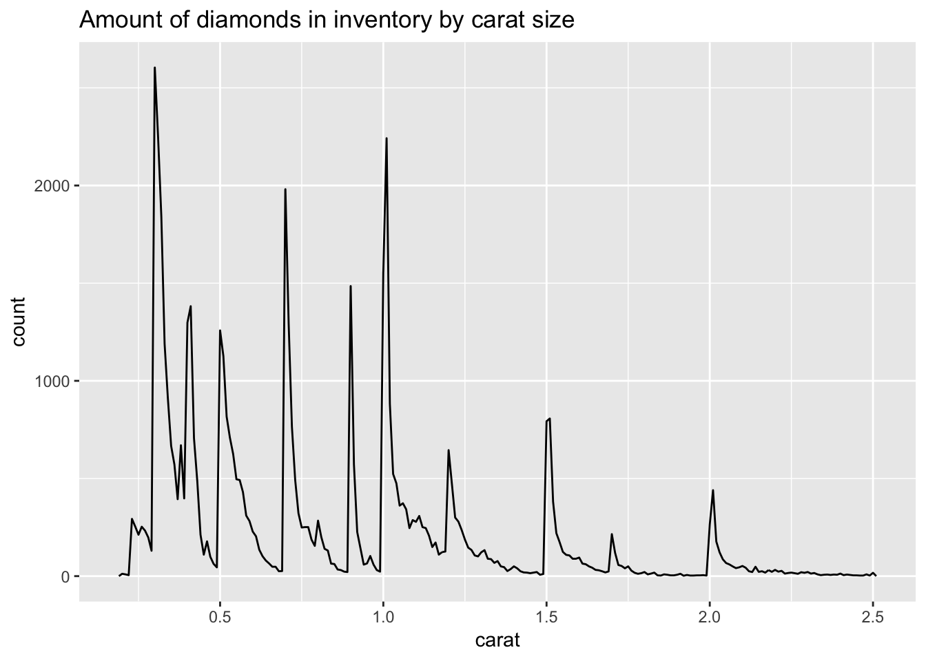
3. Copy and paste the contents of diamond-sizes.Rmd from https://github.com/hadley/r4ds/tree/master/rmarkdown in to a local R markdown document. Check that you can run it, then add text after the frequency polygon that describes its most striking features.

Below are the contents of diamond-sizes.Rmd.

smaller <- diamonds %>% 
  filter(carat <= 2.5)

We have data about 53940 diamonds. Only 126 are larger than 2.5 carats. The distribution of the remainder is shown below:

Here is my commentary on the output:

From the graph, we observe immediately that there are spikes along the frequency polygon, representing diamonds of a specific carat that are over-represented in the dataset. Looking closely, we observe that the spikes lie where there are “round” values of carat size, such as 0.5, 1, 1.5, etc. It is likely that this is a result of human rounding tendencies.

27.4.7 Exercises

1. Add a section that explores how diamond sizes vary by cut, colour, and clarity. Assume you’re writing a report for someone who doesn’t know R, and instead of setting echo = FALSE on each chunk, set a global option.

To set a global option to hide code chunks, we can include the following code chunk:

knitr::opts_chunk$set(
  echo = FALSE
)

For the learning experiences of you readers out there, I will continue to display the code that generates the graphs that explore how diamond sizes vary by cut, colour, and clarity.

# diamond size by cut
diamonds %>% ggplot (aes(x = cut, y = carat))+
  geom_boxplot()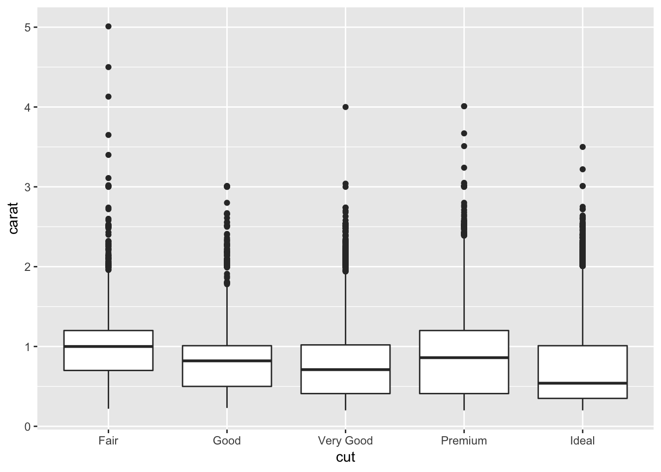

# diamond size by colour
diamonds %>% ggplot (aes(x = color, y = carat))+
  geom_boxplot()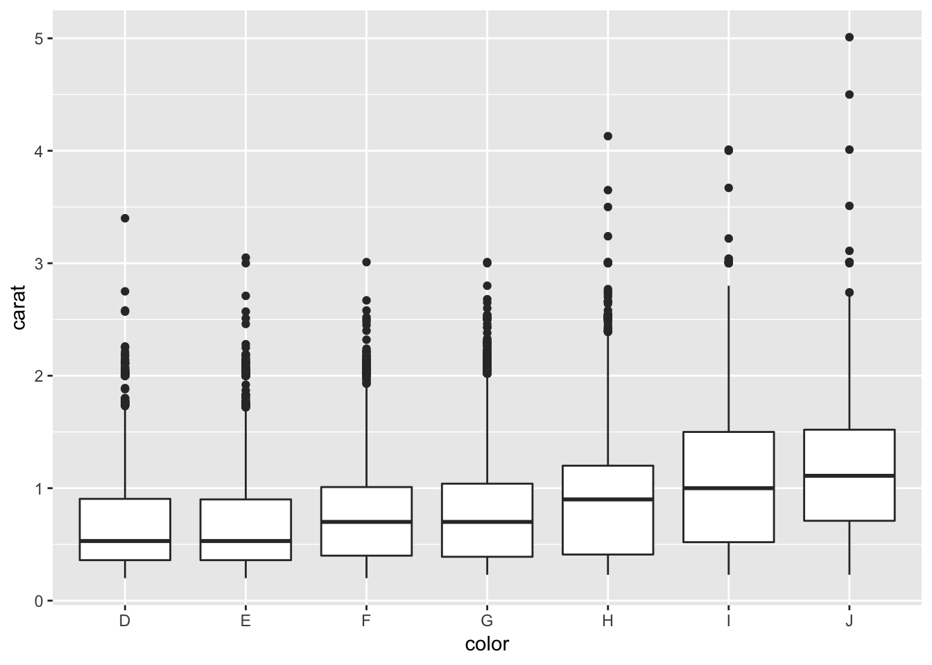

# diamond size by clarity
diamonds %>% ggplot (aes(x = clarity, y = carat))+
  geom_boxplot()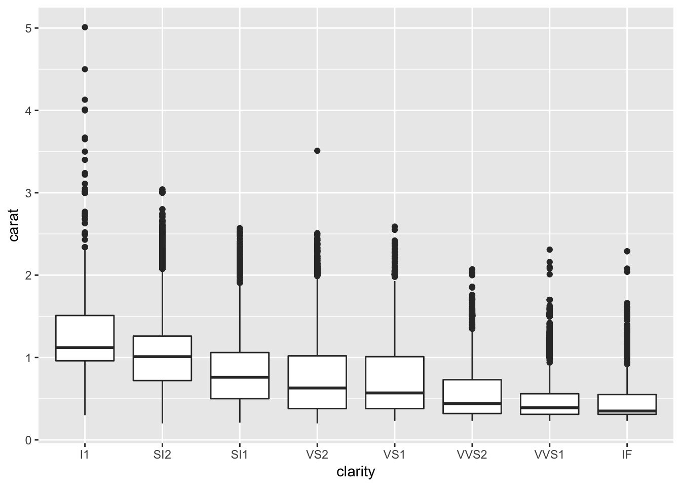

2. Download diamond-sizes.Rmd from https://github.com/hadley/r4ds/tree/master/rmarkdown. Add a section that describes the largest 20 diamonds, including a table that displays their most important attributes.

To filter out the top 20 largest diamonds, we can arrange the data table using arrange() so that the largest diamonds are at the top, then take the first 20 entries using head(). To display a table with their most important attributes, we can use knitr::kable() for carat, cut, color, clarity, and price, which I believe to be important based on the qualities they convey about the diamond.

# filter out the largest 20 diamonds

largest <- diamonds %>% arrange(desc(carat)) %>% head (20)

# display a table, using kable() to make it prettier

largest %>% select (carat, cut, color, clarity, price) %>% knitr::kable (caption = "important qualities of top 20 diamonds")

Table 1: important qualities of top 20 diamonds

carat	cut	color	clarity	price
5.01	Fair	J	I1	18018
4.50	Fair	J	I1	18531
4.13	Fair	H	I1	17329
4.01	Premium	I	I1	15223
4.01	Premium	J	I1	15223
4.00	Very Good	I	I1	15984
3.67	Premium	I	I1	16193
3.65	Fair	H	I1	11668
3.51	Premium	J	VS2	18701
3.50	Ideal	H	I1	12587
3.40	Fair	D	I1	15964
3.24	Premium	H	I1	12300
3.22	Ideal	I	I1	12545
3.11	Fair	J	I1	9823
3.05	Premium	E	I1	10453
3.04	Very Good	I	SI2	15354
3.04	Premium	I	SI2	18559
3.02	Fair	I	I1	10577
3.01	Premium	I	I1	8040
3.01	Premium	F	I1	9925

3. Modify diamonds-sizes.Rmd to use comma() to produce nicely formatted output. Also include the percentage of diamonds that are larger than 2.5 carats.

Below is the formatted output, using the comma() function specified in the chapter with an additional sentence stating the percentage of diamonds that are larger than 2.5 carats (the new sentence is bolded).

comma <- function(x) format(x, digits = 2, big.mark = ",")

smaller <- diamonds %>% 
  filter(carat <= 2.5)

We have data about 53,940 diamonds. Only 126 are larger than 2.5 carats. The percentage of diamonds that are larger than 2.5 carats is 0.2335929%. The distribution of the remainder is shown below:

4. Set up a network of chunks where d depends on c and b, and both b and c depend on a. Have each chunk print lubridate::now(), set cache = TRUE, then verify your understanding of caching.

a_variable <- 2
print(paste("a:", a_variable))

## [1] "a: 2"

lubridate::now()

## [1] "2020-01-21 21:48:01 PST"

b_variable <- 5 * a_variable
print(paste("b:", b_variable))

## [1] "b: 10"

lubridate::now()

## [1] "2020-01-21 21:48:01 PST"

c_variable <- 10 * a_variable
print(paste("c:", c_variable))

## [1] "c: 20"

lubridate::now()

## [1] "2020-01-21 21:48:01 PST"

d_product <- b_variable * c_variable
print(paste("d:", d_product))

## [1] "d: 200"

lubridate::now()

## [1] "2020-01-21 21:48:01 PST"

The output of these code chunks will be cached since we set cache = TRUE. If we re-knit this document without changing anything in the code chunks, the value of lubridate::now() that is printed to the screen should not change, since the cached values will be used.