Chapter 19 - Functions
19.2.1 Exercises
1. Why is TRUE not a parameter to rescale01()? What would happen if x contained a single missing value, and na.rm was FALSE?
TRUE is not a parameter to rescale01() because it is an option for one of the arguments in the range() function. It can be specified within the function itself rather than having to be passed in as a function parameter. If na.rm was FALSE, NA values would not be “removed” from the analysis, and the function would produce a vector of NA values. Below, I show an example what would happen if na.rm was FALSE and a vector with an NA value was used.
rescale01 <- function(x) {
  rng <- range(x, na.rm = TRUE)
  (x - rng[1]) / (rng[2] - rng[1])
}

rescale01_FALSE <- function(x) {
  rng <- range(x, na.rm = FALSE)
  (x - rng[1]) / (rng[2] - rng[1])
}

test <- c(1,2,3,NA,4,5)

rescale01(test)
## [1] 0.00 0.25 0.50 NA 0.75 1.00rescale01_FALSE(test)## [1] NA NA NA NA NA NA2. In the second variant of rescale01(), infinite values are left unchanged. Rewrite rescale01() so that -Inf is mapped to 0, and Inf is mapped to 1.
To map Inf to 1 and -Inf to 0, we can search for the indicies which have these values and assign 0 or 1 accordingly, using the which() function in base R. We then return the modified vector using return().
x <- c(1:10,Inf, c(1:3), Inf, c(1:5), -Inf)
rescale01_mapInf <- function(x) {
rng <- range(x, na.rm = TRUE, finite = TRUE)
x <- (x - rng[1]) / (rng[2] - rng[1])
x[which(x==Inf)] <- 1
x[which(x==-Inf)] <- 0
return (x)
}
rescale01_mapInf(x)
## [1] 0.0000000 0.1111111 0.2222222 0.3333333 0.4444444 0.5555556 0.6666667
## [8] 0.7777778 0.8888889 1.0000000 1.0000000 0.0000000 0.1111111 0.2222222
## [15] 1.0000000 0.0000000 0.1111111 0.2222222 0.3333333 0.4444444 0.00000003. Practice turning the following code snippets into functions. Think about what each function does. What would you call it? How many arguments does it need? Can you rewrite it to be more expressive or less duplicative?
mean(is.na(x)) is a snippet that calculates what proportion of the values in a vector are NA values. is.na(x) will return a boolean for each value in x (FALSE if not NA, TRUE if NA). TRUE is 1 and FALSE is 0 when used in mean().
x = c(1:5, NA, 1:2, NA, 1:3)
mean(is.na(x))
## [1] 0.1666667# rewrite the snippet into a function
proportion_na <- function (x) {
sum(is.na(x))/length(x)
}
# see if the function output matches the snippet
proportion_na(x)## [1] 0.1666667x / sum(x, na.rm = TRUE) is a snippet that divides each of the values in X by the total sum of the non-NA values in x.
x / sum(x, na.rm = TRUE)## [1] 0.04166667 0.08333333 0.12500000 0.16666667 0.20833333 NA
## [7] 0.04166667 0.08333333 NA 0.04166667 0.08333333 0.12500000divide_by_sum <- function (x) {
x / sum(x, na.rm = TRUE)
}
divide_by_sum(x)## [1] 0.04166667 0.08333333 0.12500000 0.16666667 0.20833333 NA
## [7] 0.04166667 0.08333333 NA 0.04166667 0.08333333 0.12500000sd(x, na.rm = TRUE) / mean(x, na.rm = TRUE) is a snippet that divides the standard deviation of the values in x by the mean of the values in x.
sd(x, na.rm = TRUE) / mean(x, na.rm = TRUE)## [1] 0.5624571sd_div_mean <- function (x) {
sd(x, na.rm = TRUE) / mean(x, na.rm = TRUE)
}
sd_div_mean(x)## [1] 0.5624571Each of the functions only requires the vector x as an input argument.
4. Follow http://nicercode.github.io/intro/writing-functions.html to write your own functions to compute the variance and skew of a numeric vector.
sample_vector <- c(1:10)

variance <- function (x) {
  n <- length(x)
    m <- mean(x)
    (1/(n - 1)) * sum((x - m)^2)
}

skew <- function (x) {
    n <- length(x)
    v <- var(x)
    m <- mean(x)
    third.moment <- (1/(n - 2)) * sum((x - m)^3)
    third.moment/(var(x)^(3/2))
}
# might have to cross-reference this function with other sources to make sure it's correct.

variance(sample_vector)
## [1] 9.166667var(sample_vector)## [1] 9.166667skew(sample_vector)## [1] 05. Write both_na(), a function that takes two vectors of the same length and returns the number of positions that have an NA in both vectors.
I interpreted this question as finding the index numbers of positions in both vectors that both contain NA values. For example, if you had one vector c(1, 2, NA, 5, 6) and another vector c(NA, 6, NA, 4, 5), this function should return “3”. To do this, we first evaluate which values in both vectors are NA values using is.na(). Then, we can use which() to find out the index of all TRUE (NA) values in these vectors. Then, we use intersect() to determine which indecies are common between the two vectors. This function should work even if the vectors are different lengths.
vector1 = c(1, 2, NA, 5, 6)
vector2 = c(NA, 6, NA, 4, 5)

both_na <- function (v1, v2) {
  na1 <- is.na(v1)
  na2 <- is.na(v2)
  intersect(which(na1==TRUE),which(na2==TRUE))
}

vector1
## [1] 1 2 NA 5 6vector2## [1] NA 6 NA 4 5both_na(vector1,vector2)## [1] 36. What do the following functions do? Why are they useful even though they are so short?
is_directory <- function(x) file.info(x)$isdir
is_readable <- function(x) file.access(x, 4) == 0
is_directory() is a function that tells the user whether the object (x) is a directory or not (returns a TRUE or FALSE value). is_readable() is a function that tells the user whether the file is readable or not (also returns TRUE or FALSE). The second argument (4) indicates that it “tests for read permission” based on the documentation. The function file.access() returns 0 for success and -1 for failure. These functions are useful because it they provide information that guides the user with how to proceed with the file.
7. Read the complete lyrics to “Little Bunny Foo Foo”. There’s a lot of duplication in this song. Extend the initial piping example to recreate the complete song, and use functions to reduce the duplication.
The lyrics are repeated three times, each time with the number of chances decreased by one. We can lump all the lyrics into one function, and then call the function 3 times using a loop while decreasing the number of chances each iteration of the loop.
# I commented out the pseudocode so the R markdown file can compile.

# foo_foo %>%
#   hop(through = forest) %>%
#   scoop(up = field_mice) %>%
#   bop(on = head) %>%
#   down(came = good_fairy) %>%
#   scoop(up = field_mice) %>%
#   bop (on = head) %>%
#   give (chances = three) %>%
#   turn (into = goonie)
#   # repeat 3 times, with the # of chances decreasing each time
#
# play_through (foo_foo, chances) {
#   hop(through = forest) %>%
#   scoop(up = field_mice) %>%
#   bop(on = head) %>%
#   down(came = good_fairy) %>%
#   scoop(up = field_mice) %>%
#   bop (on = head) %>%
#   give (chances = three) %>%
#   turn (into = goonie)
# }
#
# chances <- 3
# while (chances > 0) {
#   play_through (foo_foo, chances)
#   chances <- chances - 1
# }
#
19.3.1 Exercises
1. Read the source code for each of the following three functions, puzzle out what they do, and then brainstorm better names.
f1 <- function(string, prefix) {
  substr(string, 1, nchar(prefix)) == prefix
}

f1("hello", "he")
## [1] TRUEf1("hello", "ell")## [1] FALSEThis function returns TRUE or FALSE depending on whether the second argument (prefix) matches the corresponding first letters in the first argument (string). A better function name would be “is_prefix”.
f2 <- function(x) {
  if (length(x) <= 1) return(NULL)
  x[-length(x)]
}
x = c(1:10)
x
## [1] 1 2 3 4 5 6 7 8 9 10f2(x)## [1] 1 2 3 4 5 6 7 8 9This is a function that deletes the last entry of the input vector, x. If the vector is of length 1 or less, the function returns NULL. A better function name would be “delete_last”.
f3 <- function(x, y) {
  rep(y, length.out = length(x))
}
x = c(1:10)
x
## [1] 1 2 3 4 5 6 7 8 9 10f3(x, 5)## [1] 5 5 5 5 5 5 5 5 5 5This is a function that returns a vector that is the same length as x, but all of its values consist of y. A better name for this function would be “rep_constant_values”. Although we are not necessarily changing the values in the input vector, but rather generating a new vector with the values “replaced”, the user can infer that the output vector consist of a constant value.
2. Take a function that you’ve written recently and spend 5 minutes brainstorming a better name for it and its arguments.
Below is an example of a task that could be optimized by writing a function instead.
library(tidyverse)

preg <- tribble(
  ~pregnant, ~male, ~female,
  "yes",     NA,    10,
  "no",      20,    12
)

# without using functions, convert the pregnant and female columns to booleans (TRUE or FALSE values).
gather(preg, sex, count, male, female) %>%
  mutate(pregnant = pregnant == "yes",
         female = sex == "female") %>%
  select(-sex)
## # A tibble: 4 x 3
## pregnant count female
## <lgl> <dbl> <lgl>
## 1 TRUE NA FALSE
## 2 FALSE 20 FALSE
## 3 TRUE 10 TRUE
## 4 FALSE 12 TRUEInstead of having to place the “==” clause in the mutate function, we can write a function to do so instead.
# write function to convert a vector of strings to TRUE or FALSE, depending on whether the values match a specified string:
string_to_boolean <- function (x, string) {
  x == string
}

# use the function to do the job
gather(preg, sex, count, male, female) %>%
  mutate(pregnant = string_to_boolean(pregnant,"yes"),
         female = string_to_boolean(sex,"female")) %>%
  select(-sex)
## # A tibble: 4 x 3
## pregnant count female
## <lgl> <dbl> <lgl>
## 1 TRUE NA FALSE
## 2 FALSE 20 FALSE
## 3 TRUE 10 TRUE
## 4 FALSE 12 TRUE3. Compare and contrast rnorm() and MASS::mvrnorm(). How could you make them more consistent?
First we can compare and contrast the type of output from the two functions by generating a list of 100 random normal values with mean 0 and SD 1 using both functions (plotted below):
plot(rnorm(100), main = "rnorm()")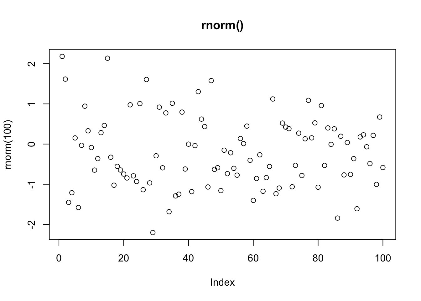
plot(MASS::mvrnorm(100,0,1), main = "MASS::mvrnorm()")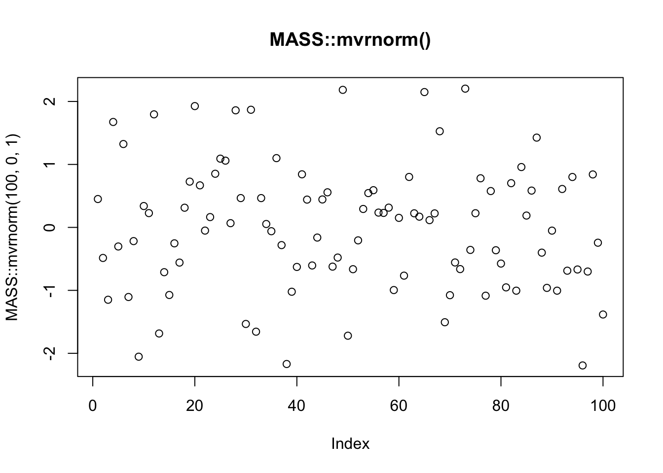
I noticed that rnorm(100) automatically sets the mean to 0 and SD to 1, whereas MASS::mvrnorm(100) does not work unless you manually specify the mean to 0 and SD to 1 in the 2nd and 3rd arguments MASS::mvrnorm(100,0,1). To make them more consistent, I would set the default values for mu and Sigma for MASS::mvrnorm() to 0 and 1, so that both functions will work without having to explicitly state the mu (mean) and Sigma (SD) values.
4. Make a case for why norm_r(), norm_d() etc would be better than rnorm(), dnorm(). Make a case for the opposite.
norm_r(), norm_d() etc would be better since you know that these functions have are common with each other in that they deal with the normal distribution. The suffix “_r“, etc lets you know how the functions differ from each other. You can also get a list of all the related functions by typing”norm" in RStudio and seeing the autocomplete options. One could argue that this is not as good as the current rnorm(), dnorm() etc convention because of the added finger work required to place an underscore in the name. Also, norm_r() is a rather cryptic name that might not have intuitive meaning, whereas rnorm immediately suggests “random normal” to one familiar with statistics.
19.4.4 Exercises
1. What’s the difference between if and ifelse()? Carefully read the help and construct three examples that illustrate the key differences.
if, if used by itself, will only execute its contents if the conditional statement is TRUE. If the statement is FALSE, nothing will be executed unless there is an else if or else statement afterwards. ifelse() gives you an option to execute code if the conditional statement is FALSE. It can also be used to filter or reassign values in a vector depending on a condition.
2. Write a greeting function that says “good morning”, “good afternoon”, or “good evening”, depending on the time of day. (Hint: use a time argument that defaults to lubridate::now(). That will make it easier to test your function.)
library(lubridate)

greet <- function ( datetime = lubridate::now() ) {
  print(datetime)
  time <- hour(datetime)

  if (time < 12) {
    print("good morning")
  } else if (time >= 12 && time < 18) {
    print("good afternoon")
  } else
    print("good evening")
}

greet()
## [1] "2020-01-21 21:47:04 PST"
## [1] "good evening"greet(ymd_hms("2016-07-08 08:34:56"))## [1] "2016-07-08 08:34:56 UTC"
## [1] "good morning"greet(ymd_hms("2016-07-08 20:34:56"))## [1] "2016-07-08 20:34:56 UTC"
## [1] "good evening"greet(ymd_hms("2016-07-08 15:34:56"))## [1] "2016-07-08 15:34:56 UTC"
## [1] "good afternoon"3. Implement a fizzbuzz function. It takes a single number as input. If the number is divisible by three, it returns “fizz”. If it’s divisible by five it returns “buzz”. If it’s divisible by three and five, it returns “fizzbuzz”. Otherwise, it returns the number. Make sure you first write working code before you create the function.
fizzbuzz <- function ( input ) {
  if (input %% 3 == 0 && input %% 5 == 0) {
    print("fizzbuzz")
  } else if ( input %% 5 == 0 ) {
    print ("buzz")
  } else if ( input %% 3 == 0 ) {
    print ("fizz")
  } else
    print (input)
}

fizzbuzz(15)
## [1] "fizzbuzz"fizzbuzz(10)## [1] "buzz"fizzbuzz(9)## [1] "fizz"fizzbuzz(4)## [1] 44. How could you use cut() to simplify this set of nested if-else statements?
# if (temp <= 0) {
#   "freezing"
# } else if (temp <= 10) {
#   "cold"
# } else if (temp <= 20) {
#   "cool"
# } else if (temp <= 30) {
#   "warm"
# } else {
#   "hot"
# }

temp_range <- c(-5:40)
# without labels
cut(temp_range, breaks = c(-100, 0, 10, 20, 30, 100), right = TRUE)
## [1] (-100,0] (-100,0] (-100,0] (-100,0] (-100,0] (-100,0] (0,10]
## [8] (0,10] (0,10] (0,10] (0,10] (0,10] (0,10] (0,10]
## [15] (0,10] (0,10] (10,20] (10,20] (10,20] (10,20] (10,20]
## [22] (10,20] (10,20] (10,20] (10,20] (10,20] (20,30] (20,30]
## [29] (20,30] (20,30] (20,30] (20,30] (20,30] (20,30] (20,30]
## [36] (20,30] (30,100] (30,100] (30,100] (30,100] (30,100] (30,100]
## [43] (30,100] (30,100] (30,100] (30,100]
## Levels: (-100,0] (0,10] (10,20] (20,30] (30,100]table(cut(temp_range, breaks = c(-100, 0, 10, 20, 30, 100), right = TRUE))##
## (-100,0] (0,10] (10,20] (20,30] (30,100]
## 6 10 10 10 10# with labels
cut(temp_range, breaks = c(-100, 0, 10, 20, 30, 100), labels = c("freezing", "cold", "cool", "warm", "hot"), right = TRUE)## [1] freezing freezing freezing freezing freezing freezing cold
## [8] cold cold cold cold cold cold cold
## [15] cold cold cool cool cool cool cool
## [22] cool cool cool cool cool warm warm
## [29] warm warm warm warm warm warm warm
## [36] warm hot hot hot hot hot hot
## [43] hot hot hot hot
## Levels: freezing cold cool warm hottable(cut(temp_range, breaks = c(-100, 0, 10, 20, 30, 100), labels = c("freezing", "cold", "cool", "warm", "hot"), right = TRUE))##
## freezing cold cool warm hot
## 6 10 10 10 10How would you change the call to cut() if I’d used < instead of <=? What is the other chief advantage of cut() for this problem? (Hint: what happens if you have many values in temp?)
If < was used instead of <=, I would change the argument from right = TRUE to right = FALSE. This will split the interval to be closed on the left and open on the right. The other advantage of cut() for this problem is that it is able to sort a vector of values into the various intervals, whereas the nested if else statement that was provided only works on a single value. This makes cut() more efficient when there are many values to be sorted into the intervals.
5. What happens if you use switch() with numeric values?
Based on the documentation for switch(), if numerical values are input for the EXPR parameter (first argument), switch() will choose the corresponding element of the list of alternatives (…). I wrote an example below. Switch(1) will choose the first argument after EXPR (the second total argument in the switch() function). If a numerical input for EXPR is larger than the number of alternatives, it seems no output is provided (typeof() returns NULL).
test_switch <- function ( x ) {
  switch(x,
         "first choice after EXPR",
         2,
         "third",
         "4th choice after EXPR"
         )
}
test_switch(1)
## [1] "first choice after EXPR"test_switch(2)## [1] 2test_switch(3)## [1] "third"test_switch(4)## [1] "4th choice after EXPR"typeof(test_switch(5))## [1] "NULL"6. What does this switch() call do? What happens if x is “e”?
Below I turn the provided switch() call into a function and test each of the possibilities for x, as well as try what happens when x is “e”. Since there is no output provided for options a or c, the switch() function returns the value immediately afterwards. So test_switch(“a”) returns the same value as test_switch(“b”), and test_switch(“c”) returns the same value as test_switch(“d”). If x is “e”, a NULL value is returned. There seems to be no output but if you use typeof(test_switch(“e”)), we see that the value is NULL.
test_switch <- function (x) {
  switch(x,
    a = ,
    b = "ab",
    c = ,
    d = "cd"
  )
}

test_switch("a")
## [1] "ab"test_switch("b")## [1] "ab"test_switch("c")## [1] "cd"test_switch("d")## [1] "cd"test_switch("e")
typeof(test_switch("e"))## [1] "NULL"19.5.5 Exercises
1. What does commas(letters, collapse = “-”) do? Why?
commas(letters, collapse = “-”) results in an error. I think the intention of the code was to combine all the letters separated by hyphens (for example, a-b-c-d-e…). In order to do this, we would have to modify the commas function directly (shown below, a new function called hyphens()). The code that was provided seems to attempt to incorrectly override the collapse argument by specifying it after letters. Since commas() has ... as its only argument, this means that collapse = “-” is incorporated into the ..., resulting in the error.
commas <- function(...) stringr::str_c(..., collapse = ", ")
commas(letters[1:10])
## [1] "a, b, c, d, e, f, g, h, i, j"# this produces an error:
# commas(letters[1:10], collapse = "-")
# to produce the intended output, modify the commas function.
hyphens <- function(...) stringr::str_c(..., collapse = "-")
hyphens(letters[1:10])## [1] "a-b-c-d-e-f-g-h-i-j"Alternatively, we could modify the function to allow the user to specify what type of insertion to use as an argument after ..., with the default being commas. I name the function insert_between(), below.
insert_between <- function(..., insert = ", ") stringr::str_c(..., collapse = insert)
insert_between (letters[1:10])
## [1] "a, b, c, d, e, f, g, h, i, j"insert_between (letters[1:10], insert = "-")## [1] "a-b-c-d-e-f-g-h-i-j"2. It’d be nice if you could supply multiple characters to the pad argument, e.g. rule(“Title”, pad = “-+”). Why doesn’t this currently work? How could you fix it?
This doesn’t currently work optimally because the rule becomes twice as long (due to there being 2 characters instead of 1 for the pad argument). To fix this, we could divide the width according to the length of the pad argument. To figure out how many characters are in pad, use nchar(). Then, divide the width parameter by this number. This results in a rule that is the appropriate length. I show what the existing function does below, along with a modified function that performs the correct result.
# The original rule function, showing what happens if multiple characters were supplied:
rule <- function(..., pad = "-") {
  title <- paste0(...)
  width <- getOption("width") - nchar(title) - 5
  cat(title, " ", stringr::str_dup(pad, width), "\n", sep = "")
}

rule("Important output")
## Important output ------------------------------------------------------rule("Title", pad = "-+")## Title -+-+-+-+-+-+-+-+-+-+-+-+-+-+-+-+-+-+-+-+-+-+-+-+-+-+-+-+-+-+-+-+-+-+-+-+-+-+-+-+-+-+-+-+-+-+-+-+-+-+-+-+-+-+-+-+-+-+-+-+-+-+-+-+-+# An improved version that scales the padding based on the character length:
scaled_rule <- function(..., pad = "-") {
title <- paste0(...)
pad_length <- nchar(pad)
print(str_c("Number of characters in pad: ", pad_length))
width <- (getOption("width") - nchar(title) - 5)/pad_length
print(str_c("Number of times pad was duplicated: ", width))
cat(title, " ", stringr::str_dup(pad, width), "\n", sep = "")
}
scaled_rule("Important output")## [1] "Number of characters in pad: 1"
## [1] "Number of times pad was duplicated: 54"
## Important output ------------------------------------------------------scaled_rule("Title", pad = "-+")## [1] "Number of characters in pad: 2"
## [1] "Number of times pad was duplicated: 32.5"
## Title -+-+-+-+-+-+-+-+-+-+-+-+-+-+-+-+-+-+-+-+-+-+-+-+-+-+-+-+-+-+-+-+3. What does the trim argument to mean() do? When might you use it?
The trim argument in mean() will remove a proportion of values from both sides of the vector before calculating the mean of the remaining values. The proportion is between 0 to 0.5, with default value being 0 (no trim applied). Examples below of how trim may affect mean calculation. You might use this when you are calculating something in which the edge cases have high variability or contain unreliable data.
x = c(1,1,1:10,1,1)
mean(x)
## [1] 4.214286mean(x, trim = 0.2)## [1] 3.84. The default value for the method argument to cor() is c(“pearson”, “kendall”, “spearman”). What does that mean? What value is used by default?
Based on the documentation for cor(), these specify the type of correlation coefficient that is calculated by the function. The default value used is “pearson”. Below is an example of how changing these parameters may affect the output, since each method uses a different equation.
x = c(1:20)
y = c(1,1,1,1:15, 5, 6)
cor(x,y)
## [1] 0.796562cor(x,y, method = "kendall")## [1] 0.7743726cor(x,y, method = "spearman")## [1] 0.8157183