Chapter 23 - Model basics
Notes - making simple models
library(tidyverse)
library(modelr)
The datasets that are used in this chapter are simulated datasets, such as the one shown below (sim1)
head(sim1)## # A tibble: 6 x 2
## x y
## <int> <dbl>
## 1 1 4.20
## 2 1 7.51
## 3 1 2.13
## 4 2 8.99
## 5 2 10.2
## 6 2 11.3Below are the functions used in this chapter, written by Hadley for demonstration purposes:
model1 <- function(a, data) {
  a[1] + data$x * a[2]
}

measure_distance <- function(mod, data) {
  diff <- data$y - model1(mod, data)
  sqrt(mean(diff ^ 2))
}

sim1_dist <- function(a1, a2) {
  measure_distance(c(a1, a2), sim1)
}

grid <- expand.grid(
  a1 = seq(-5, 20, length = 25),
  a2 = seq(1, 3, length = 25)
  ) %>%
  mutate(dist = purrr::map2_dbl(a1, a2, sim1_dist))

head(grid)
## a1 a2 dist
## 1 -5.0000000 1 15.45248
## 2 -3.9583333 1 14.44317
## 3 -2.9166667 1 13.43881
## 4 -1.8750000 1 12.44058
## 5 -0.8333333 1 11.45009
## 6 0.2083333 1 10.46955dim(grid)## [1] 625 3grid %>%
ggplot(aes(a1, a2)) +
geom_point(data = filter(grid, rank(dist) <= 10), size = 4, colour = "red") +
geom_point(aes(colour = -dist))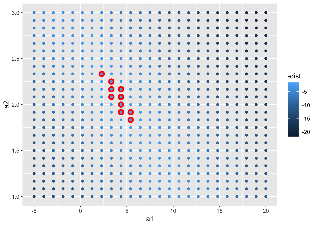
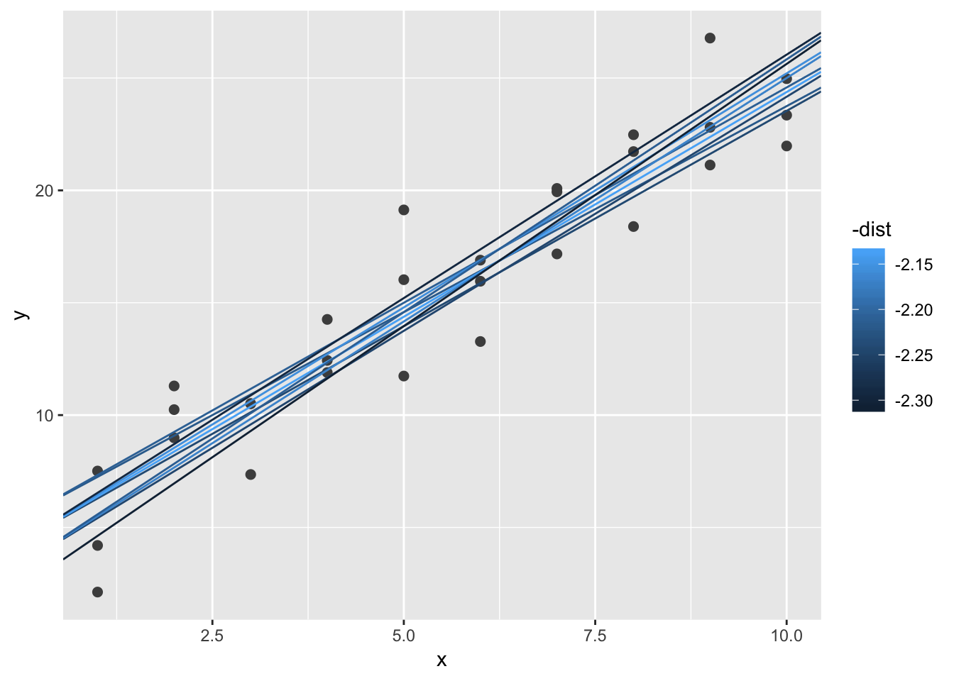
ggplot(sim1, aes(x, y)) +
  geom_point(size = 2, colour = "grey30") +
  geom_abline(
    aes(intercept = a1, slope = a2, colour = -dist),
    data = filter(grid, rank(dist) <= 10)
  )
23.2.1 Exercises
1. One downside of the linear model is that it is sensitive to unusual values because the distance incorporates a squared term. Fit a linear model to the simulated data below, and visualise the results. Rerun a few times to generate different simulated datasets. What do you notice about the model?
In the simulated dataset, there are a couple of outliers that are far displaced from the rest of the points. These outliers can skew the linear approximation, because these points are so ‘distant’ from the other points in the dataset. Because the linear model tries to minimize the distance between each point and the fitted model (the “residuals”), these outliers will skew the approximation, pulling the line closer to them. The larger the residual, the more it contributes to the RMSE. We notice that the fitted line is slightly skewed towards the direction of the outlying point.
sim1a <- tibble(
  x = rep(1:10, each = 3),
  y = x * 1.5 + 6 + rt(length(x), df = 2)
)

# first, take a look at the data
sim1a
## # A tibble: 30 x 2
## x y
## <int> <dbl>
## 1 1 7.18
## 2 1 8.82
## 3 1 6.37
## 4 2 10.5
## 5 2 8.93
## 6 2 7.69
## 7 3 11.3
## 8 3 9.12
## 9 3 10.5
## 10 4 9.71
## # … with 20 more rowsggplot(sim1a, aes (x, y)) +
geom_point()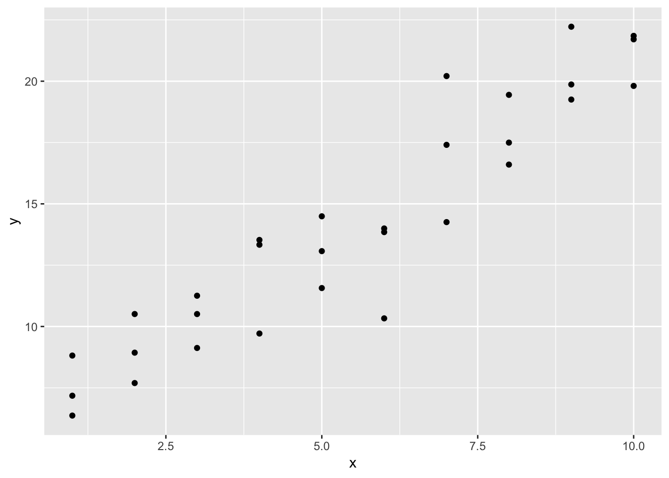
mod <- lm(y~x, data = sim1a)
summary(mod)##
## Call:
## lm(formula = y ~ x, data = sim1a)
##
## Residuals:
## Min 1Q Median 3Q Max
## -4.5890 -1.0620 0.1046 1.0860 3.7401
##
## Coefficients:
## Estimate Std. Error t value Pr(>|t|)
## (Intercept) 5.6279 0.6715 8.381 4.07e-09 ***
## x 1.5487 0.1082 14.310 2.10e-14 ***
## ---
## Signif. codes: 0 '***' 0.001 '**' 0.01 '*' 0.05 '.' 0.1 ' ' 1
##
## Residual standard error: 1.703 on 28 degrees of freedom
## Multiple R-squared: 0.8797, Adjusted R-squared: 0.8754
## F-statistic: 204.8 on 1 and 28 DF, p-value: 2.105e-14# add the fitted linear model to the scatterplot
ggplot(sim1a, aes (x, y)) +
geom_point()+
geom_abline(intercept = mod$coefficients[1], slope = mod$coefficients[2])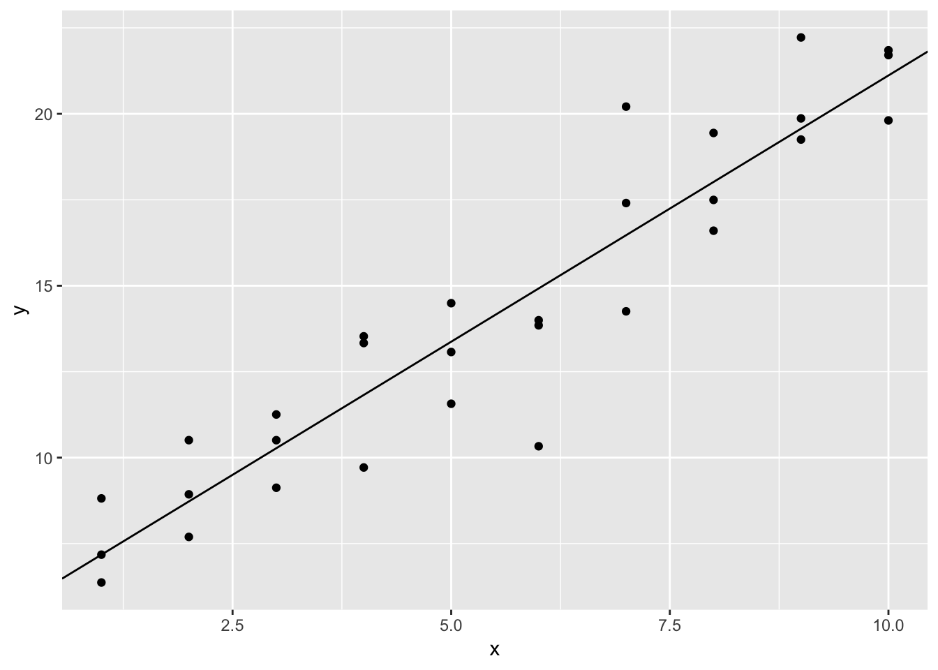
# compare with the baseR lm with geom_smooth() overlay, looks like they overlap, as expected
ggplot(sim1a, aes (x, y)) +
  geom_point()+
  geom_abline(intercept = mod$coefficients[1], slope = mod$coefficients[2], size=3, color = "red")+
  geom_smooth(method = 'lm')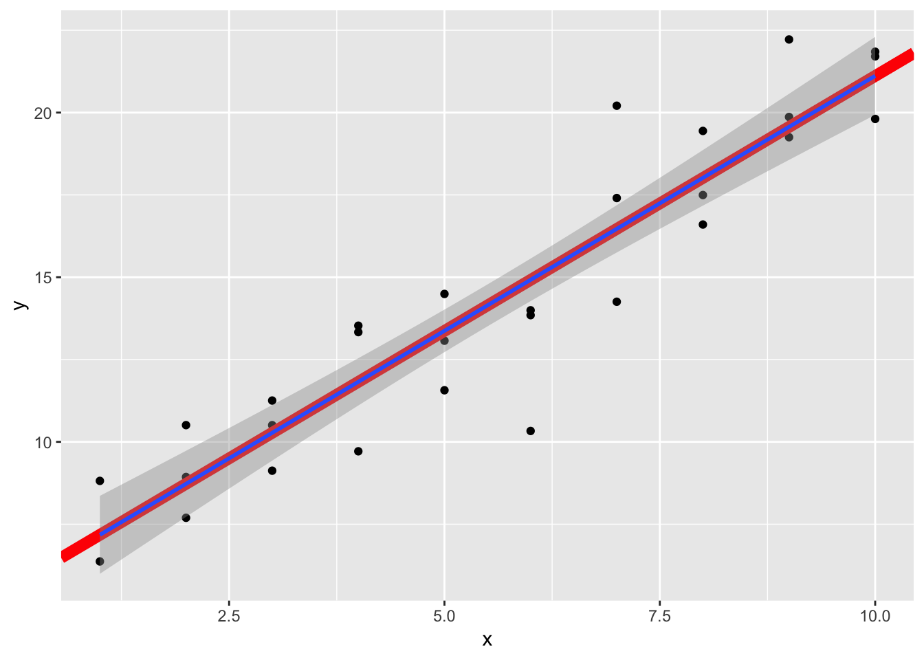
2. One way to make linear models more robust is to use a different distance measure. For example, instead of root-mean-squared distance, you could use mean-absolute distance:
measure_distance <- function(mod, data) {
  diff <- data$y - model1(mod, data)
  mean(abs(diff))
}
# use optim() function to
best <- optim(c(0, 0), measure_distance, data = sim1a)
best$par
## [1] 5.592108 1.586087# compare the parameters from optim() with the parameters obtained from lm()
mod <- lm (y~x, data = sim1a)
coef(mod)## (Intercept) x
## 5.627914 1.548750# plot the two lines on the scatterplot to observe differences in fit
ggplot(data = sim1a, aes(x, y))+
geom_point()+
geom_abline(slope = mod$coefficients[2], intercept = mod$coefficients[1], color = "red")+
geom_abline(slope = best$par[2], intercept = best$par[1], color = "blue")+
labs(title = "Red = root-mean-squared distance fit using lm() \n Blue = mean-absolute distance fit using optim()")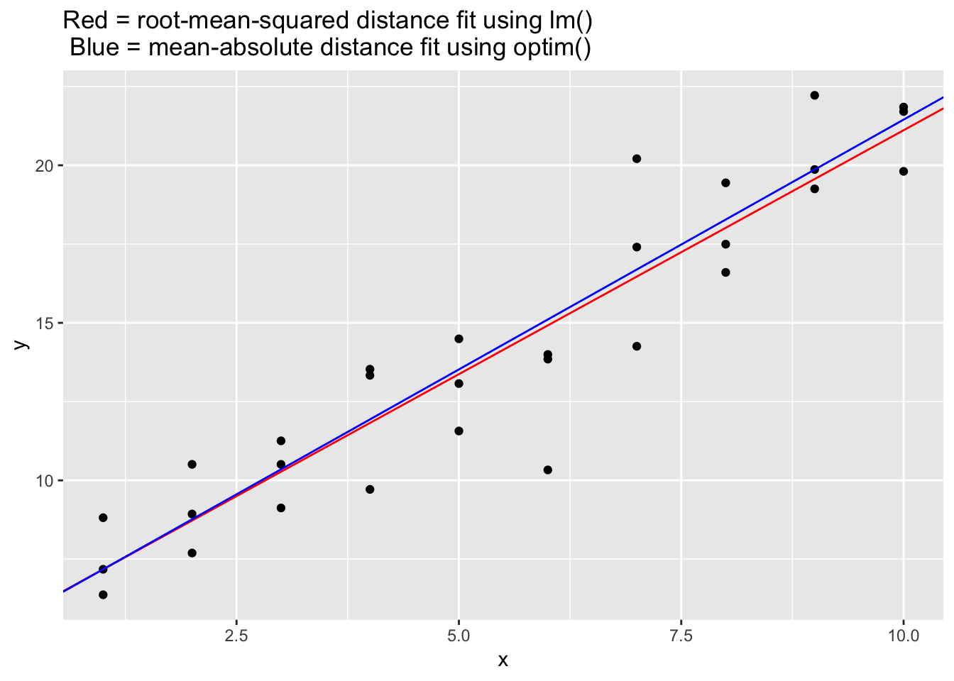
Use optim() to fit this model to the simulated data above and compare it to the linear model.
The measure_distance() function provided above uses the absolute-mean distance (mean(abs(diff))) instead of the root-mean-squared distance, sqrt(mean(diff^2)). Using optim() and the absolute-mean distance, we find that the line is less skewed by the outlying points. The red line is “pulled” more towards the outliers, whereas the blue line remains more embbeded with the bulk of the data. This is because squaring the residuals results in much greater values when the residuals are large, so minimizing the residuals for outliers takes more priority when using the squared distance.
3. One challenge with performing numerical optimisation is that it’s only guaranteed to find one local optimum. What’s the problem with optimising a three parameter model like this?
A quadratic or higher order function may have more than one local minimum / maximum. This may result in the optim() function providing an unideal result. In the provided function, since a[1] and a[3] are both constants that are not multiplied by a column in data (such as data$x), they can be added together and represent the intercept of the line. This results in the sum of a[1] and a[3] equalling the intercept we found before using the equation a[1] + data$x * a[2].
a[1] and a[3] can therefore have infinite possibilites of values, as long as the sum of a[1] and a[3] are equal to the local optimum of a[1] + data$x * a[2]. In the example below, if we use the dataset sim1, we find that a[1] and a[3] must sum to 4.220074. So, depending on where you start with the optim() function, a[1] and a[3] will have differing values, but still add up to 4.220074.
We see in the graph that the optim() function and lm() again provde the same result.
model1 <- function(a, data) {
  a[1] + data$x * a[2] + a[3]
}

measure_distance <- function(mod, data) {
  diff <- data$y - model1(mod, data)
  sqrt(mean(diff ^ 2))
}

best <- optim(c(0, 0, 0), measure_distance, data = sim1)
best$par
## [1] 3.3672228 2.0515737 0.8528513best <- optim(c(0, 0, 1), measure_distance, data = sim1)
best$par## [1] -3.469885 2.051509 7.690289# since in the model above, a[1] and a[3] may be theoretically combined to represent the intercept of the line, we can graph it as such:
ggplot(data = sim1, aes(x, y))+
geom_point()+
geom_smooth(method = "lm", color = "red", size = 2)+
geom_abline(slope = best$par[2], intercept = best$par[1] + best$par[3], color = "blue")+
labs(title = "Red = using lm() \n Blue = optim() using the provided 3 parameter model")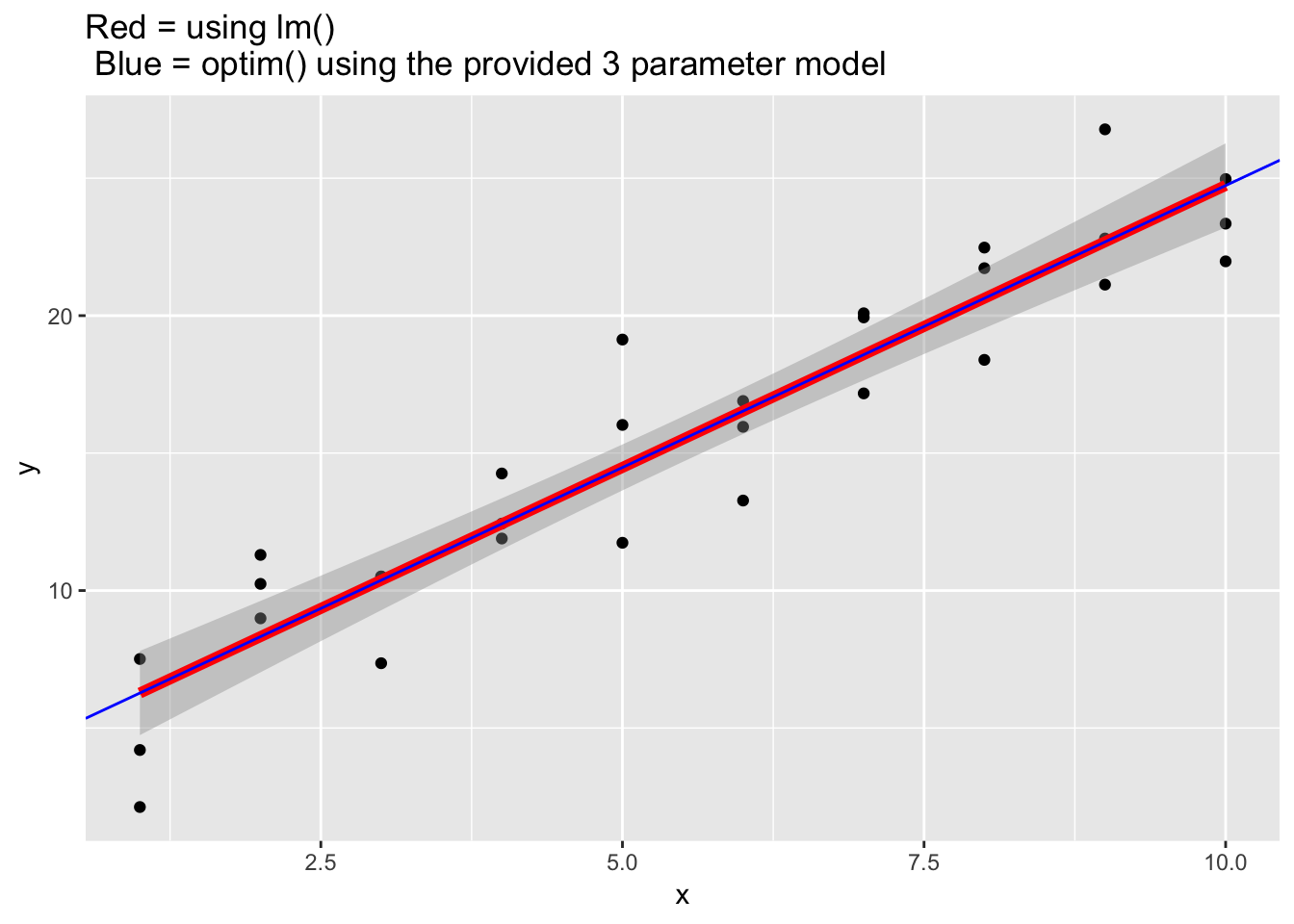
23.3.3 Exercises
1. Instead of using lm() to fit a straight line, you can use loess() to fit a smooth curve. Repeat the process of model fitting, grid generation, predictions, and visualisation on sim1 using loess() instead of lm(). How does the result compare to geom_smooth()?
Using the loess() function instead of lm(), the line curves more towards the direction of variation and is not strictly a straight line. The default method for fitting using geom_smooth() is loess(), so the line that is superimposed on the ggplot is the same as the line generated by the predictions using the loess() model. When we superimpose all 3 options (loess() prediction, lm() prediction, and geom_smooth()), we see that geom_smooth() and the loess() prediction precisely overlap, whereas the lm() prediction does not.
# using lm()
sim1_mod_lm <- lm(y ~ x, data = sim1)

grid <- sim1 %>%
  data_grid(x)
grid
## # A tibble: 10 x 1
## x
## <int>
## 1 1
## 2 2
## 3 3
## 4 4
## 5 5
## 6 6
## 7 7
## 8 8
## 9 9
## 10 10grid <- grid %>%
add_predictions(sim1_mod_lm)
grid## # A tibble: 10 x 2
## x pred
## <int> <dbl>
## 1 1 6.27
## 2 2 8.32
## 3 3 10.4
## 4 4 12.4
## 5 5 14.5
## 6 6 16.5
## 7 7 18.6
## 8 8 20.6
## 9 9 22.7
## 10 10 24.7sim1 <- sim1 %>%
add_residuals(sim1_mod_lm)
sim1## # A tibble: 30 x 3
## x y resid
## <int> <dbl> <dbl>
## 1 1 4.20 -2.07
## 2 1 7.51 1.24
## 3 1 2.13 -4.15
## 4 2 8.99 0.665
## 5 2 10.2 1.92
## 6 2 11.3 2.97
## 7 3 7.36 -3.02
## 8 3 10.5 0.130
## 9 3 10.5 0.136
## 10 4 12.4 0.00763
## # … with 20 more rowsggplot(sim1, aes(x)) +
geom_point(aes(y = y)) +
geom_line(aes(y = pred), data = grid, colour = "red", size = 1)
ggplot(sim1, aes(x, resid)) +
geom_ref_line(h = 0) +
geom_point() 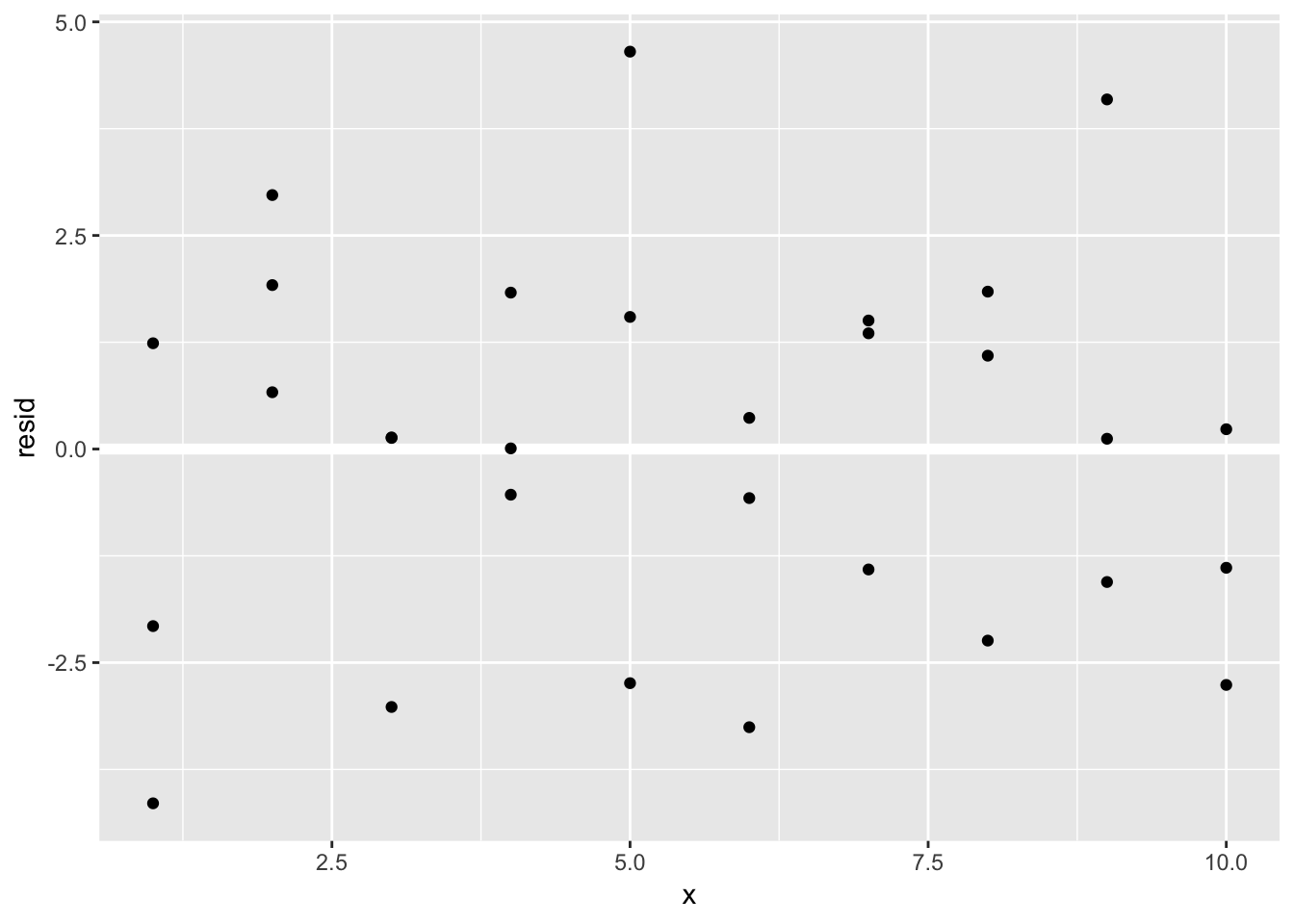
# using loess()
sim1_mod_loess <- loess(y ~ x, data = sim1)
grid <- sim1 %>%
data_grid(x)
grid## # A tibble: 10 x 1
## x
## <int>
## 1 1
## 2 2
## 3 3
## 4 4
## 5 5
## 6 6
## 7 7
## 8 8
## 9 9
## 10 10grid <- grid %>%
add_predictions(sim1_mod_loess)
grid## # A tibble: 10 x 2
## x pred
## <int> <dbl>
## 1 1 5.34
## 2 2 8.27
## 3 3 10.8
## 4 4 12.8
## 5 5 14.6
## 6 6 16.6
## 7 7 18.7
## 8 8 20.8
## 9 9 22.6
## 10 10 24.0sim1 <- sim1 %>%
add_residuals(sim1_mod_loess)
sim1## # A tibble: 30 x 3
## x y resid
## <int> <dbl> <dbl>
## 1 1 4.20 -1.14
## 2 1 7.51 2.17
## 3 1 2.13 -3.21
## 4 2 8.99 0.714
## 5 2 10.2 1.97
## 6 2 11.3 3.02
## 7 3 7.36 -3.45
## 8 3 10.5 -0.304
## 9 3 10.5 -0.298
## 10 4 12.4 -0.345
## # … with 20 more rows# residuals plot
ggplot(sim1, aes(x, resid)) +
geom_ref_line(h = 0) +
geom_point() 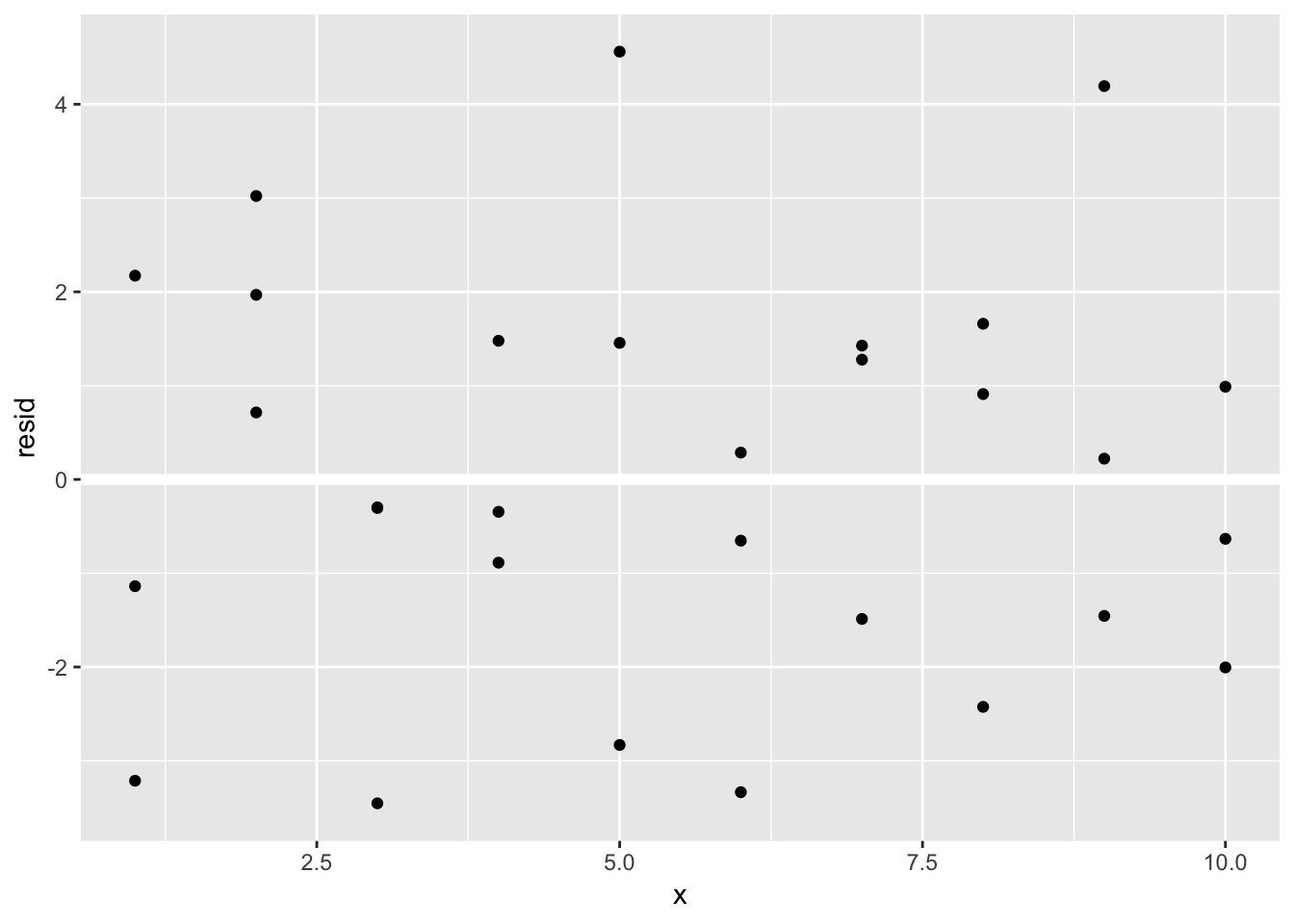
# plot the regression line
ggplot(sim1, aes(x)) +
  geom_point(aes(y = y)) +
  geom_line(aes(y = pred), data = grid, colour = "red", size = 1)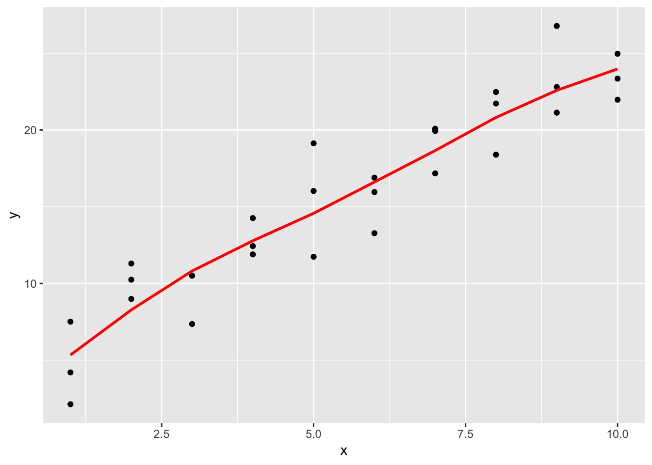
# compare to geom_smooth() and lm()
ggplot(sim1, aes(x, y)) +
  geom_point() +
  geom_line(aes(y = pred), data = grid, colour = "red", size = 3)+
  geom_smooth(color = "blue", se = F)+
  geom_smooth(method = "lm", color = "green", se = F)
## `geom_smooth()` using method = 'loess' and formula 'y ~ x'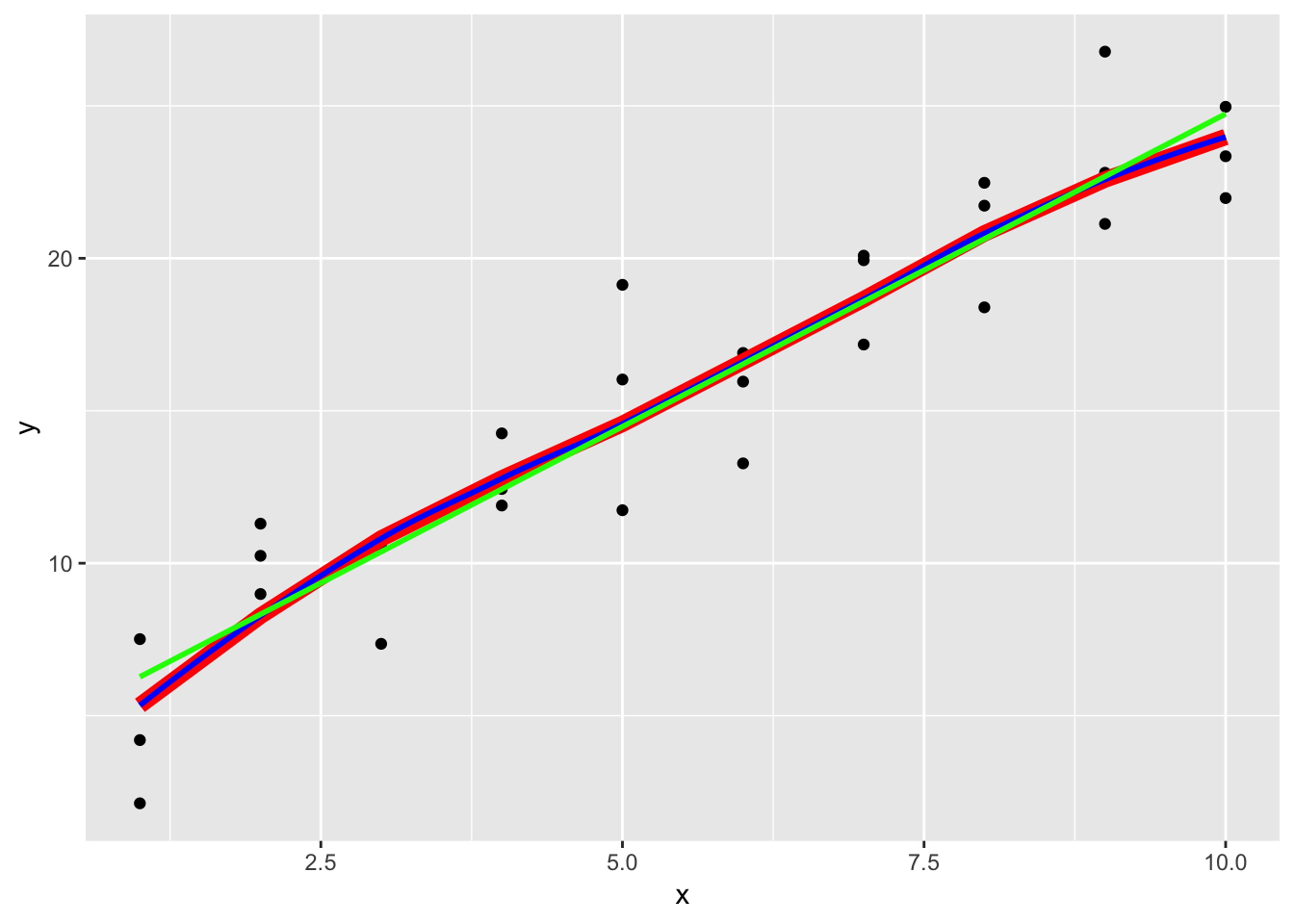
2. add_predictions() is paired with gather_predictions() and spread_predictions(). How do these three functions differ?
add_predictions() can only work with one supplied model, in which it will generate a new column named “pred” in your data frame. gather_predictions() and spread_predictions() can work with multiple supplied models and generate predictions for each model supplied. gather_predictions() appends the model name to the data frame along with the predictions as new rows to the data frame, in a tidy fashion. spread_predictions() appends the new predictions to the data frame as separate columns. You can visualize the differences below, in which spread_predictions makes the data frame “wider” and gather_predictions() makes the data frame “taller”.
grid <- sim1 %>%
  data_grid(x)
grid
## # A tibble: 10 x 1
## x
## <int>
## 1 1
## 2 2
## 3 3
## 4 4
## 5 5
## 6 6
## 7 7
## 8 8
## 9 9
## 10 10grid_add <- grid %>%
add_predictions(sim1_mod_lm)
grid_add## # A tibble: 10 x 2
## x pred
## <int> <dbl>
## 1 1 6.27
## 2 2 8.32
## 3 3 10.4
## 4 4 12.4
## 5 5 14.5
## 6 6 16.5
## 7 7 18.6
## 8 8 20.6
## 9 9 22.7
## 10 10 24.7grid_gather <- grid %>%
gather_predictions(sim1_mod_lm, sim1_mod_loess)
grid_gather## # A tibble: 20 x 3
## model x pred
## <chr> <int> <dbl>
## 1 sim1_mod_lm 1 6.27
## 2 sim1_mod_lm 2 8.32
## 3 sim1_mod_lm 3 10.4
## 4 sim1_mod_lm 4 12.4
## 5 sim1_mod_lm 5 14.5
## 6 sim1_mod_lm 6 16.5
## 7 sim1_mod_lm 7 18.6
## 8 sim1_mod_lm 8 20.6
## 9 sim1_mod_lm 9 22.7
## 10 sim1_mod_lm 10 24.7
## 11 sim1_mod_loess 1 5.34
## 12 sim1_mod_loess 2 8.27
## 13 sim1_mod_loess 3 10.8
## 14 sim1_mod_loess 4 12.8
## 15 sim1_mod_loess 5 14.6
## 16 sim1_mod_loess 6 16.6
## 17 sim1_mod_loess 7 18.7
## 18 sim1_mod_loess 8 20.8
## 19 sim1_mod_loess 9 22.6
## 20 sim1_mod_loess 10 24.0grid_spread <- grid %>%
spread_predictions(sim1_mod_lm, sim1_mod_loess)
grid_spread## # A tibble: 10 x 3
## x sim1_mod_lm sim1_mod_loess
## <int> <dbl> <dbl>
## 1 1 6.27 5.34
## 2 2 8.32 8.27
## 3 3 10.4 10.8
## 4 4 12.4 12.8
## 5 5 14.5 14.6
## 6 6 16.5 16.6
## 7 7 18.6 18.7
## 8 8 20.6 20.8
## 9 9 22.7 22.6
## 10 10 24.7 24.03. What does geom_ref_line() do? What package does it come from? Why is displaying a reference line in plots showing residuals useful and important?
geom_ref_line() adds either a horizontal or vertical line at a specified position to your ggplot, of a specified color (default white). It comes from modelr. This is useful when plotting residuals because ideally the residuals should be centered around 0. Having a reference line helps the viewer judge how the residuals behave. Conceptually, we can think of the horizontal line in the residuals plot as the prediction, and of the residual as how far off the true value is from that prediction.
4. Why might you want to look at a frequency polygon of absolute residuals? What are the pros and cons compared to looking at the raw residuals?
The residuals, ideally, should approximately be normally distributed. Examining the frequency polygon is useful as a visual assessment for whether or not the residuals follow the Normal distribution. This graph will also more easily capture any abnormal pattern in the residuals, in which there are over-representations of either + or - residuals. The cons are that this graph masks some of the variability in the residuals by binning them, and you lose the relationship between the residual and the predictor variable. This is best paired with a scatterplot of the residuals so you can observe exactly where each point lies in relation to the predictor variable.
# example from book
ggplot(sim1, aes(resid)) +
  geom_freqpoly(binwidth = 0.5)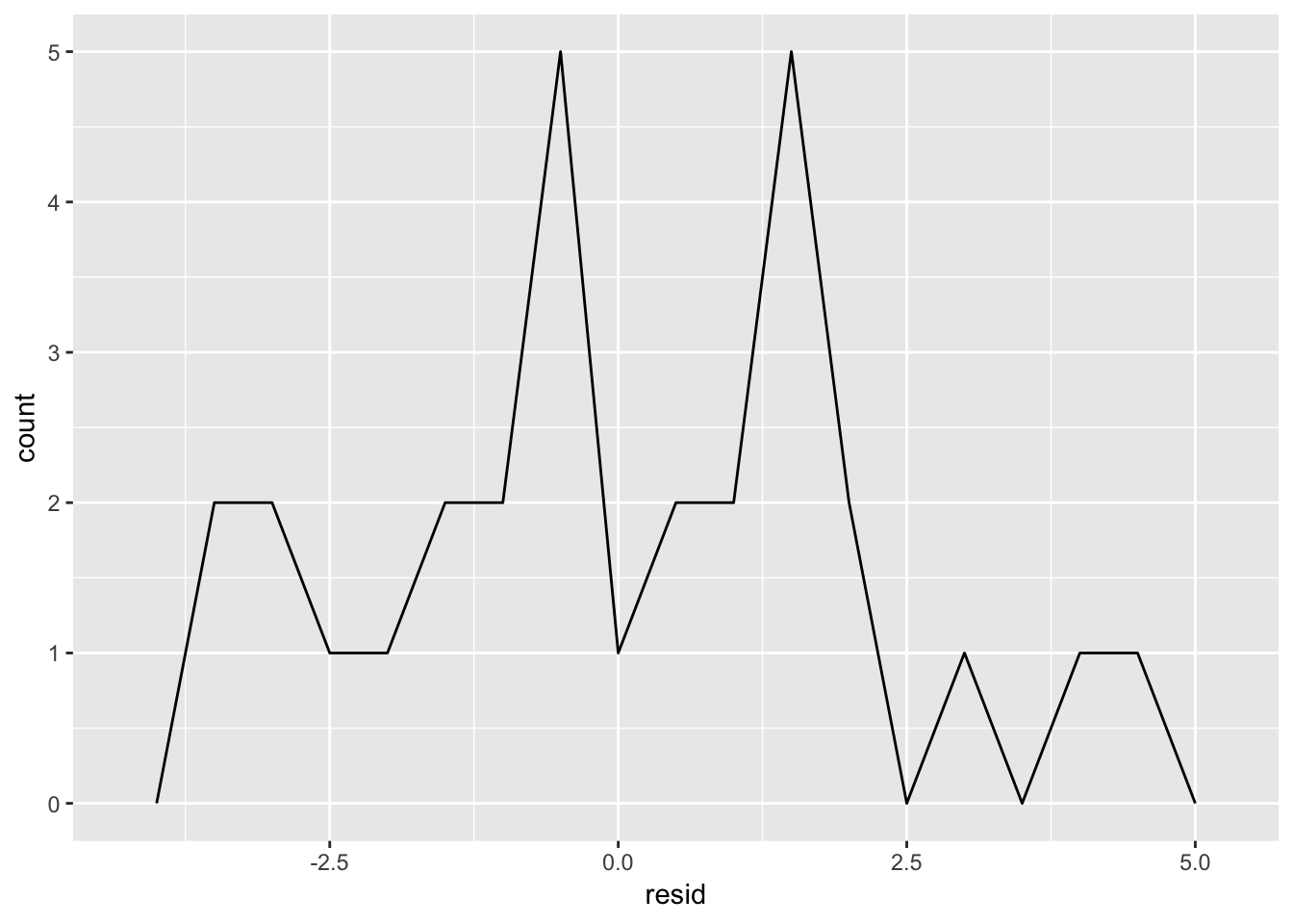
# make an example where residuals approximate normal distribution
x = seq(1:1000)
y = 12 + 5 * x + rnorm(1000,0,100) # add random white noise
mysim <- as_tibble(cbind(x, y))

#fit model
mysim_mod <- lm(y ~ x, data = mysim)
summary(mysim_mod)
##
## Call:
## lm(formula = y ~ x, data = mysim)
##
## Residuals:
## Min 1Q Median 3Q Max
## -297.929 -70.571 -0.186 72.620 296.649
##
## Coefficients:
## Estimate Std. Error t value Pr(>|t|)
## (Intercept) 15.14761 6.47572 2.339 0.0195 *
## x 5.00035 0.01121 446.146 <2e-16 ***
## ---
## Signif. codes: 0 '***' 0.001 '**' 0.01 '*' 0.05 '.' 0.1 ' ' 1
##
## Residual standard error: 102.3 on 998 degrees of freedom
## Multiple R-squared: 0.995, Adjusted R-squared: 0.995
## F-statistic: 1.99e+05 on 1 and 998 DF, p-value: < 2.2e-16# make predictions
mygrid <- mysim %>%
data_grid(x)
mygrid## # A tibble: 1,000 x 1
## x
## <dbl>
## 1 1
## 2 2
## 3 3
## 4 4
## 5 5
## 6 6
## 7 7
## 8 8
## 9 9
## 10 10
## # … with 990 more rowsmygrid <- mygrid %>% add_predictions(mysim_mod)
mygrid## # A tibble: 1,000 x 2
## x pred
## <dbl> <dbl>
## 1 1 20.1
## 2 2 25.1
## 3 3 30.1
## 4 4 35.1
## 5 5 40.1
## 6 6 45.1
## 7 7 50.2
## 8 8 55.2
## 9 9 60.2
## 10 10 65.2
## # … with 990 more rowsmysim <- mysim %>% add_residuals(mysim_mod)
mysim## # A tibble: 1,000 x 3
## x y resid
## <dbl> <dbl> <dbl>
## 1 1 110. 89.4
## 2 2 45.6 20.5
## 3 3 162. 132.
## 4 4 78.7 43.6
## 5 5 -9.92 -50.1
## 6 6 135. 90.3
## 7 7 -151. -201.
## 8 8 94.4 39.3
## 9 9 162. 101.
## 10 10 -39.7 -105.
## # … with 990 more rows# plot prediction line
ggplot(mysim, aes(x)) +
geom_point(aes(y = y)) +
geom_line(aes(y = pred), data = mygrid, colour = "red", size = 1)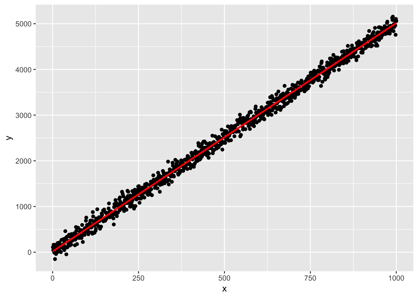
# plot freqpoly() of residuals
ggplot(mysim, aes(resid)) +
  geom_freqpoly()
## `stat_bin()` using `bins = 30`. Pick better value with `binwidth`.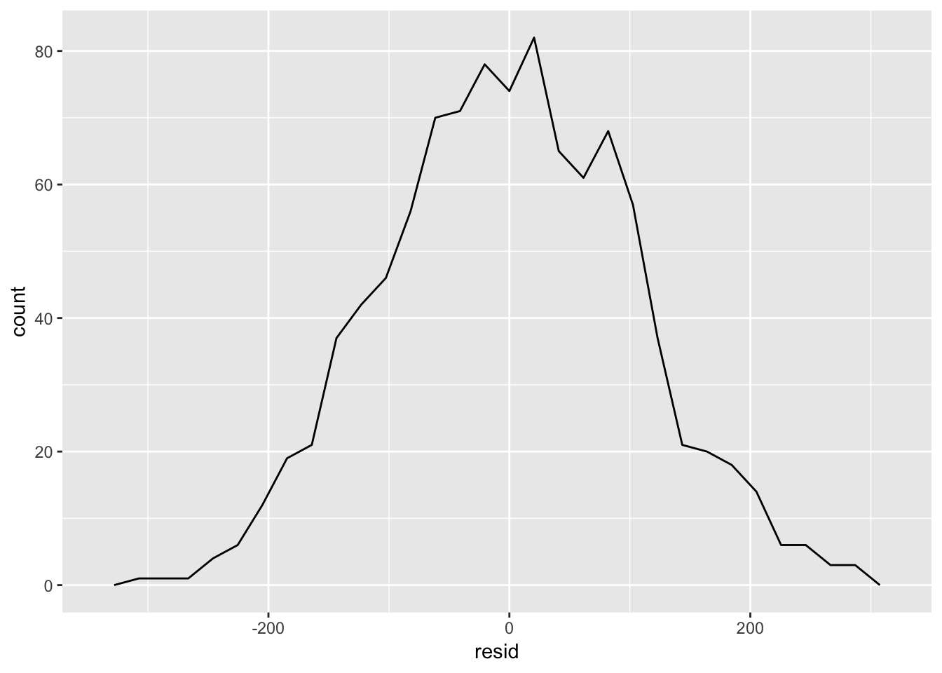
# plot scatterplot of residuals
ggplot(mysim, aes (x = x, y = resid))+
  geom_ref_line(h=0)+
  geom_point()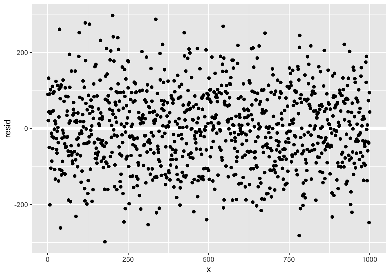
23.4.5 Exercises
For categorical variables, the book performs a similar prediction workflow:
# use the sim2 dataset from modelr
sim2
## # A tibble: 40 x 2
## x y
## <chr> <dbl>
## 1 a 1.94
## 2 a 1.18
## 3 a 1.24
## 4 a 2.62
## 5 a 1.11
## 6 a 0.866
## 7 a -0.910
## 8 a 0.721
## 9 a 0.687
## 10 a 2.07
## # … with 30 more rows# examine how the data are distributed
ggplot(sim2) +
geom_point(aes(x, y))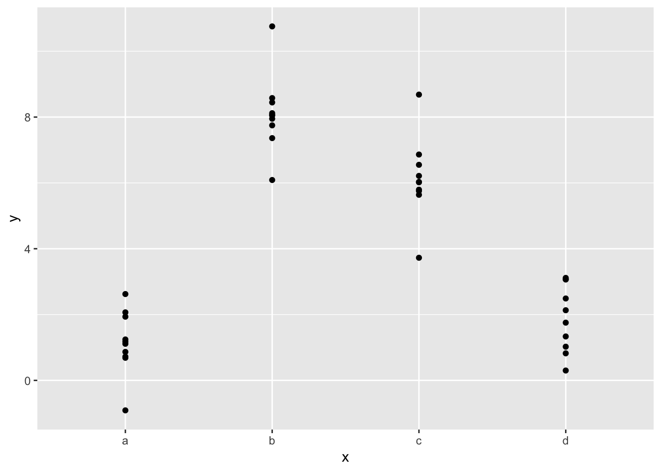
# generate a model (R automatically recognizes that the predictor variables are categorical)
mod2 <- lm(y ~ x, data = sim2)

# generate predictions based on model
grid <- sim2 %>%
  data_grid(x) %>%
  add_predictions(mod2)
grid
## # A tibble: 4 x 2
## x pred
## <chr> <dbl>
## 1 a 1.15
## 2 b 8.12
## 3 c 6.13
## 4 d 1.91# plot the predictions overlaid on the graph
ggplot(sim2, aes(x)) +
geom_point(aes(y = y)) +
geom_point(data = grid, aes(y = pred), colour = "red", size = 4)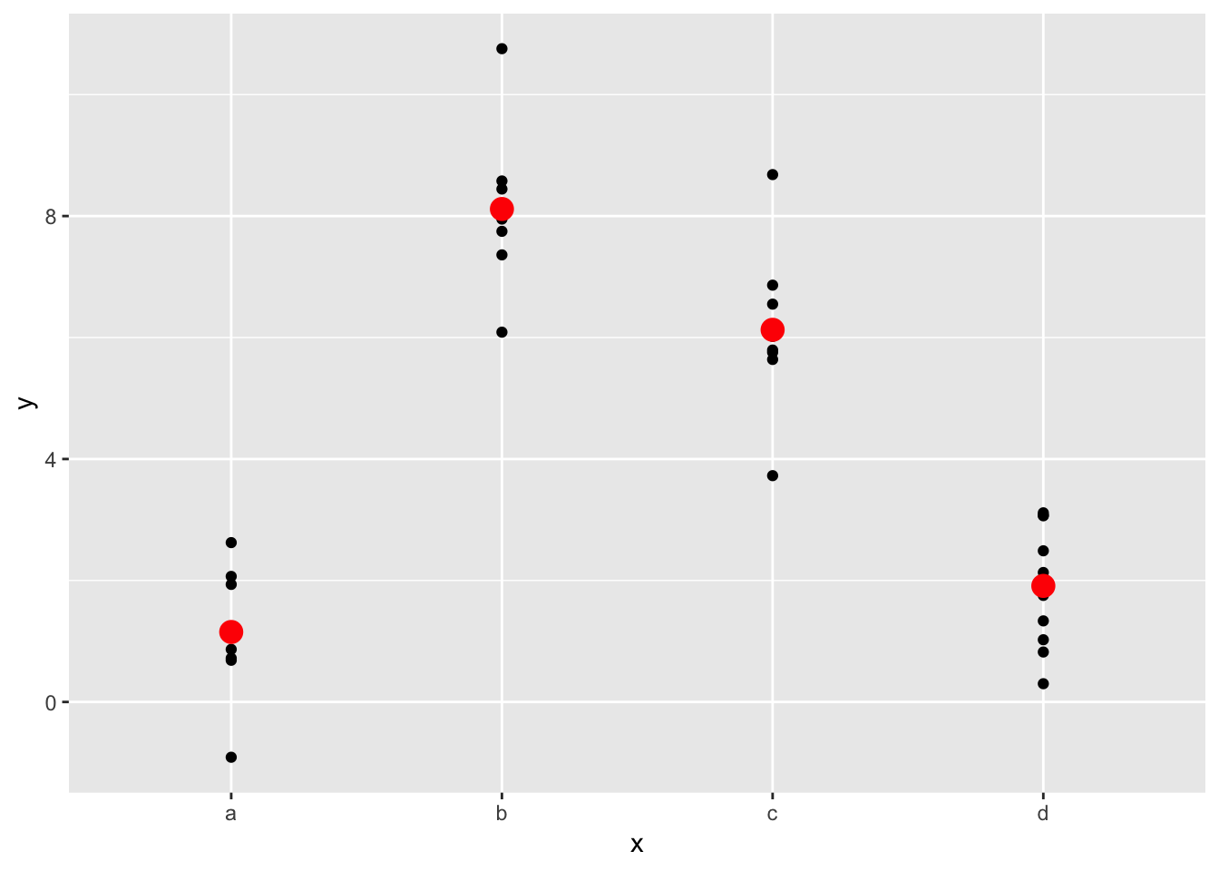
For using more than one predictor variable (can be a combination of categorical and continuous variables), a similar approach is used:
# examine data and build models
sim3
## # A tibble: 120 x 5
## x1 x2 rep y sd
## <int> <fct> <int> <dbl> <dbl>
## 1 1 a 1 -0.571 2
## 2 1 a 2 1.18 2
## 3 1 a 3 2.24 2
## 4 1 b 1 7.44 2
## 5 1 b 2 8.52 2
## 6 1 b 3 7.72 2
## 7 1 c 1 6.51 2
## 8 1 c 2 5.79 2
## 9 1 c 3 6.07 2
## 10 1 d 1 2.11 2
## # … with 110 more rowsmod1 <- lm(y ~ x1 + x2, data = sim3)
mod2 <- lm(y ~ x1 * x2, data = sim3)
# inputting multiple variables into data_grid results in it returning all the possible combinations between x1 and x2
grid <- sim3 %>%
data_grid(x1, x2) %>%
gather_predictions(mod1, mod2)
grid## # A tibble: 80 x 4
## model x1 x2 pred
## <chr> <int> <fct> <dbl>
## 1 mod1 1 a 1.67
## 2 mod1 1 b 4.56
## 3 mod1 1 c 6.48
## 4 mod1 1 d 4.03
## 5 mod1 2 a 1.48
## 6 mod1 2 b 4.37
## 7 mod1 2 c 6.28
## 8 mod1 2 d 3.84
## 9 mod1 3 a 1.28
## 10 mod1 3 b 4.17
## # … with 70 more rowsInputting multiple continuous variables into data_grid will also return all possible combinations, unless you manually specify the combinations as done in the book chapter.
# examine data and build models
sim4
## # A tibble: 300 x 4
## x1 x2 rep y
## <dbl> <dbl> <int> <dbl>
## 1 -1 -1 1 4.25
## 2 -1 -1 2 1.21
## 3 -1 -1 3 0.353
## 4 -1 -0.778 1 -0.0467
## 5 -1 -0.778 2 4.64
## 6 -1 -0.778 3 1.38
## 7 -1 -0.556 1 0.975
## 8 -1 -0.556 2 2.50
## 9 -1 -0.556 3 2.70
## 10 -1 -0.333 1 0.558
## # … with 290 more rowsmod1 <- lm(y ~ x1 + x2, data = sim4)
mod2 <- lm(y ~ x1 * x2, data = sim4)
# with manual specification of range
grid <- sim4 %>%
data_grid(
x1 = seq_range(x1, 5),
x2 = seq_range(x2, 5)
) %>%
gather_predictions(mod1, mod2)
grid## # A tibble: 50 x 4
## model x1 x2 pred
## <chr> <dbl> <dbl> <dbl>
## 1 mod1 -1 -1 0.996
## 2 mod1 -1 -0.5 -0.395
## 3 mod1 -1 0 -1.79
## 4 mod1 -1 0.5 -3.18
## 5 mod1 -1 1 -4.57
## 6 mod1 -0.5 -1 1.91
## 7 mod1 -0.5 -0.5 0.516
## 8 mod1 -0.5 0 -0.875
## 9 mod1 -0.5 0.5 -2.27
## 10 mod1 -0.5 1 -3.66
## # … with 40 more rows# without manual specification of range, provides all combinations of values
grid2 <- sim4 %>%
data_grid(
x1,
x2
)
grid2## # A tibble: 100 x 2
## x1 x2
## <dbl> <dbl>
## 1 -1 -1
## 2 -1 -0.778
## 3 -1 -0.556
## 4 -1 -0.333
## 5 -1 -0.111
## 6 -1 0.111
## 7 -1 0.333
## 8 -1 0.556
## 9 -1 0.778
## 10 -1 1
## # … with 90 more rows1. What happens if you repeat the analysis of sim2 using a model without an intercept. What happens to the model equation? What happens to the predictions?
To fit a model to sim2 without an intercept, use “-1” with the formula, as shown. We observe that the model matrix loses the “intercept” column when we use “-1”. We then generate predictions using gather_predictions() on both models. We find that both models generate the same predictions! This is because in both cases, the mean of the observations for each categorical possibility is the optimal fit.
mod1 <- lm(y ~ x, data = sim2)
model_matrix(sim2, y ~x)
## # A tibble: 40 x 4
## `(Intercept)` xb xc xd
## <dbl> <dbl> <dbl> <dbl>
## 1 1 0 0 0
## 2 1 0 0 0
## 3 1 0 0 0
## 4 1 0 0 0
## 5 1 0 0 0
## 6 1 0 0 0
## 7 1 0 0 0
## 8 1 0 0 0
## 9 1 0 0 0
## 10 1 0 0 0
## # … with 30 more rowsmod2 <- lm(y ~ x - 1, data = sim2)
model_matrix(sim2, y ~x -1)## # A tibble: 40 x 4
## xa xb xc xd
## <dbl> <dbl> <dbl> <dbl>
## 1 1 0 0 0
## 2 1 0 0 0
## 3 1 0 0 0
## 4 1 0 0 0
## 5 1 0 0 0
## 6 1 0 0 0
## 7 1 0 0 0
## 8 1 0 0 0
## 9 1 0 0 0
## 10 1 0 0 0
## # … with 30 more rowsgrid <- sim2 %>%
data_grid(x) %>%
gather_predictions(mod1, mod2)
grid## # A tibble: 8 x 3
## model x pred
## <chr> <chr> <dbl>
## 1 mod1 a 1.15
## 2 mod1 b 8.12
## 3 mod1 c 6.13
## 4 mod1 d 1.91
## 5 mod2 a 1.15
## 6 mod2 b 8.12
## 7 mod2 c 6.13
## 8 mod2 d 1.91ggplot(sim2, aes(x)) +
geom_point(aes(y = y)) +
geom_point(data = grid, aes(y = pred, shape = model, color = model), size = 4)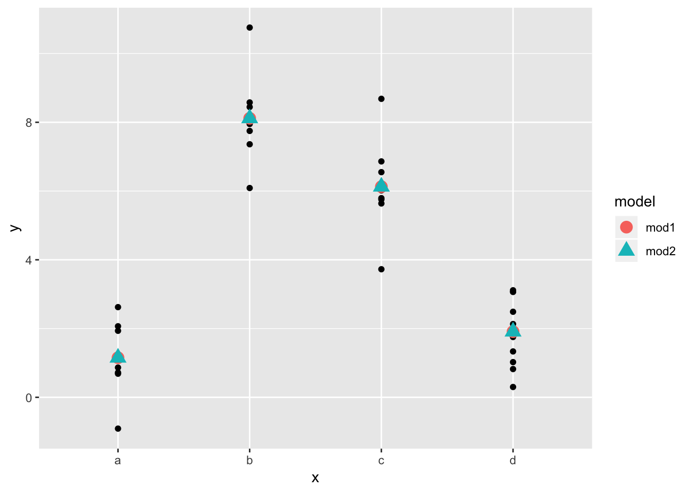
2. Use model_matrix() to explore the equations generated for the models I fit to sim3 and sim4. Why is * a good shorthand for interaction?
The model matrix for y ~ x1 + x2 for sim3 has an intercept, an x1 column, and 3 columns for x2, corresponding to each of the possibilities for the categories in x2. The model matrix for y ~ x1 * x2 has an these columns as well, but also has x1:x2b, x1:x2c, and x1:x2d, which correspond to the interaction between x1 and each of the categories in x2.
For sim4, since the values of the predictor variables x1 and x2 are both continuous variables, the x2 column does not need to be split up as in sim3. The model matrix consists of 3 columns, an intercept, x1, and x2. Similarly, y ~ x1 * x2 uses a model matrix of 4 columns, which consists of the 3 mentioned previously and an additional column x1:x2.
is a good shorthand for this interaction because the additional columns that it adds are products. it suggests that changes in values of one variable will affect the value of the other, which is what it is trying to model.
sim3## # A tibble: 120 x 5
## x1 x2 rep y sd
## <int> <fct> <int> <dbl> <dbl>
## 1 1 a 1 -0.571 2
## 2 1 a 2 1.18 2
## 3 1 a 3 2.24 2
## 4 1 b 1 7.44 2
## 5 1 b 2 8.52 2
## 6 1 b 3 7.72 2
## 7 1 c 1 6.51 2
## 8 1 c 2 5.79 2
## 9 1 c 3 6.07 2
## 10 1 d 1 2.11 2
## # … with 110 more rows# models fit to sim3
model_matrix(sim3, y ~ x1 + x2 )## # A tibble: 120 x 5
## `(Intercept)` x1 x2b x2c x2d
## <dbl> <dbl> <dbl> <dbl> <dbl>
## 1 1 1 0 0 0
## 2 1 1 0 0 0
## 3 1 1 0 0 0
## 4 1 1 1 0 0
## 5 1 1 1 0 0
## 6 1 1 1 0 0
## 7 1 1 0 1 0
## 8 1 1 0 1 0
## 9 1 1 0 1 0
## 10 1 1 0 0 1
## # … with 110 more rowsmodel_matrix(sim3, y ~ x1 * x2 )## # A tibble: 120 x 8
## `(Intercept)` x1 x2b x2c x2d `x1:x2b` `x1:x2c` `x1:x2d`
## <dbl> <dbl> <dbl> <dbl> <dbl> <dbl> <dbl> <dbl>
## 1 1 1 0 0 0 0 0 0
## 2 1 1 0 0 0 0 0 0
## 3 1 1 0 0 0 0 0 0
## 4 1 1 1 0 0 1 0 0
## 5 1 1 1 0 0 1 0 0
## 6 1 1 1 0 0 1 0 0
## 7 1 1 0 1 0 0 1 0
## 8 1 1 0 1 0 0 1 0
## 9 1 1 0 1 0 0 1 0
## 10 1 1 0 0 1 0 0 1
## # … with 110 more rowssim4## # A tibble: 300 x 4
## x1 x2 rep y
## <dbl> <dbl> <int> <dbl>
## 1 -1 -1 1 4.25
## 2 -1 -1 2 1.21
## 3 -1 -1 3 0.353
## 4 -1 -0.778 1 -0.0467
## 5 -1 -0.778 2 4.64
## 6 -1 -0.778 3 1.38
## 7 -1 -0.556 1 0.975
## 8 -1 -0.556 2 2.50
## 9 -1 -0.556 3 2.70
## 10 -1 -0.333 1 0.558
## # … with 290 more rows# models fit to sim4
model_matrix(sim4, y ~ x1 + x2 )## # A tibble: 300 x 3
## `(Intercept)` x1 x2
## <dbl> <dbl> <dbl>
## 1 1 -1 -1
## 2 1 -1 -1
## 3 1 -1 -1
## 4 1 -1 -0.778
## 5 1 -1 -0.778
## 6 1 -1 -0.778
## 7 1 -1 -0.556
## 8 1 -1 -0.556
## 9 1 -1 -0.556
## 10 1 -1 -0.333
## # … with 290 more rowsmodel_matrix(sim4, y ~ x1 * x2 )## # A tibble: 300 x 4
## `(Intercept)` x1 x2 `x1:x2`
## <dbl> <dbl> <dbl> <dbl>
## 1 1 -1 -1 1
## 2 1 -1 -1 1
## 3 1 -1 -1 1
## 4 1 -1 -0.778 0.778
## 5 1 -1 -0.778 0.778
## 6 1 -1 -0.778 0.778
## 7 1 -1 -0.556 0.556
## 8 1 -1 -0.556 0.556
## 9 1 -1 -0.556 0.556
## 10 1 -1 -0.333 0.333
## # … with 290 more rows3. Using the basic principles, convert the formulas in the following two models into functions. (Hint: start by converting the categorical variable into 0-1 variables.)
The formulas below use the model matricies that were described in exercise 2 of this section. We can re-create the model matricies by writing a function that accepts the predictor variables as input, as well as the type of operator. In the example below, I input sim3 along with either “+” or “*” and show that the model matricies generated match those made by the modelr function model_matrix().
mod1 <- lm(y ~ x1 + x2, data = sim3)
mod2 <- lm(y ~ x1 * x2, data = sim3)

# check to see if the column to add is a categorical variable (factor), and split it up if true
add_column <- function ( mycolumn, colname ) {
  # test whether the columns are factors or not
  if (is.factor (mycolumn)){
    my_levels <- levels(mycolumn)

    # split into separate columns
    output <- vector("list")
    for (i in 2: length(my_levels)) {
      level_name <- str_c(colname, my_levels[i])
      output[[level_name]] <- 1*(mycolumn == my_levels[i])
    }
  }
  # if not factor, return the column as-is
  else {
    output <- list( mycolumn)
    names(output) <- colname
  }
  output
}

# check the type of operator supplied (+ or *) and create the columns as necessary, calling the add_column function
make_matrix <- function (data, operator) {
  my_colnames <- c("x1", "x2")
  # store the columns of the model matrix in "mm"
  mm <- list()

  # make the default intercept column
  mm$intercept <- rep(1, length(data$x2))

  # add the base columns using add_column()
  for (item in my_colnames) {
    mm <- c(mm, add_column (data[[item]], item))
  }
  mm <- bind_cols(mm)

  # if the operator is *, add the appropriate columns based on vector multiplication
  if (operator == "*") {
    x1cols <- colnames(mm)[grep("x1", colnames(mm))]
    x2cols <- colnames(mm)[grep("x2", colnames(mm))]
    newcols <- vector("list")
    for (i in x1cols) {
      print(i)
      for (j in x2cols) {
        print(j)
        new_level_name <- str_c(i,j, sep = ":")
        print(new_level_name)
        newcols[[new_level_name]] <- mm[[i]]* mm[[j]]
      }
    }
    newcols <- bind_cols(newcols)
    mm <- cbind(mm, newcols)
  }
  mm
}

make_matrix( sim3, "+")
## # A tibble: 120 x 5
## intercept x1 x2b x2c x2d
## <dbl> <int> <dbl> <dbl> <dbl>
## 1 1 1 0 0 0
## 2 1 1 0 0 0
## 3 1 1 0 0 0
## 4 1 1 1 0 0
## 5 1 1 1 0 0
## 6 1 1 1 0 0
## 7 1 1 0 1 0
## 8 1 1 0 1 0
## 9 1 1 0 1 0
## 10 1 1 0 0 1
## # … with 110 more rowsmodel_matrix( sim3, y ~ x1 + x2)## # A tibble: 120 x 5
## `(Intercept)` x1 x2b x2c x2d
## <dbl> <dbl> <dbl> <dbl> <dbl>
## 1 1 1 0 0 0
## 2 1 1 0 0 0
## 3 1 1 0 0 0
## 4 1 1 1 0 0
## 5 1 1 1 0 0
## 6 1 1 1 0 0
## 7 1 1 0 1 0
## 8 1 1 0 1 0
## 9 1 1 0 1 0
## 10 1 1 0 0 1
## # … with 110 more rowsmake_matrix( sim3, "*")## [1] "x1"
## [1] "x2b"
## [1] "x1:x2b"
## [1] "x2c"
## [1] "x1:x2c"
## [1] "x2d"
## [1] "x1:x2d"## intercept x1 x2b x2c x2d x1:x2b x1:x2c x1:x2d
## 1 1 1 0 0 0 0 0 0
## 2 1 1 0 0 0 0 0 0
## 3 1 1 0 0 0 0 0 0
## 4 1 1 1 0 0 1 0 0
## 5 1 1 1 0 0 1 0 0
## 6 1 1 1 0 0 1 0 0
## 7 1 1 0 1 0 0 1 0
## 8 1 1 0 1 0 0 1 0
## 9 1 1 0 1 0 0 1 0
## 10 1 1 0 0 1 0 0 1
## 11 1 1 0 0 1 0 0 1
## 12 1 1 0 0 1 0 0 1
## 13 1 2 0 0 0 0 0 0
## 14 1 2 0 0 0 0 0 0
## 15 1 2 0 0 0 0 0 0
## 16 1 2 1 0 0 2 0 0
## 17 1 2 1 0 0 2 0 0
## 18 1 2 1 0 0 2 0 0
## 19 1 2 0 1 0 0 2 0
## 20 1 2 0 1 0 0 2 0
## 21 1 2 0 1 0 0 2 0
## 22 1 2 0 0 1 0 0 2
## 23 1 2 0 0 1 0 0 2
## 24 1 2 0 0 1 0 0 2
## 25 1 3 0 0 0 0 0 0
## 26 1 3 0 0 0 0 0 0
## 27 1 3 0 0 0 0 0 0
## 28 1 3 1 0 0 3 0 0
## 29 1 3 1 0 0 3 0 0
## 30 1 3 1 0 0 3 0 0
## 31 1 3 0 1 0 0 3 0
## 32 1 3 0 1 0 0 3 0
## 33 1 3 0 1 0 0 3 0
## 34 1 3 0 0 1 0 0 3
## 35 1 3 0 0 1 0 0 3
## 36 1 3 0 0 1 0 0 3
## 37 1 4 0 0 0 0 0 0
## 38 1 4 0 0 0 0 0 0
## 39 1 4 0 0 0 0 0 0
## 40 1 4 1 0 0 4 0 0
## 41 1 4 1 0 0 4 0 0
## 42 1 4 1 0 0 4 0 0
## 43 1 4 0 1 0 0 4 0
## 44 1 4 0 1 0 0 4 0
## 45 1 4 0 1 0 0 4 0
## 46 1 4 0 0 1 0 0 4
## 47 1 4 0 0 1 0 0 4
## 48 1 4 0 0 1 0 0 4
## 49 1 5 0 0 0 0 0 0
## 50 1 5 0 0 0 0 0 0
## 51 1 5 0 0 0 0 0 0
## 52 1 5 1 0 0 5 0 0
## 53 1 5 1 0 0 5 0 0
## 54 1 5 1 0 0 5 0 0
## 55 1 5 0 1 0 0 5 0
## 56 1 5 0 1 0 0 5 0
## 57 1 5 0 1 0 0 5 0
## 58 1 5 0 0 1 0 0 5
## 59 1 5 0 0 1 0 0 5
## 60 1 5 0 0 1 0 0 5
## 61 1 6 0 0 0 0 0 0
## 62 1 6 0 0 0 0 0 0
## 63 1 6 0 0 0 0 0 0
## 64 1 6 1 0 0 6 0 0
## 65 1 6 1 0 0 6 0 0
## 66 1 6 1 0 0 6 0 0
## 67 1 6 0 1 0 0 6 0
## 68 1 6 0 1 0 0 6 0
## 69 1 6 0 1 0 0 6 0
## 70 1 6 0 0 1 0 0 6
## 71 1 6 0 0 1 0 0 6
## 72 1 6 0 0 1 0 0 6
## 73 1 7 0 0 0 0 0 0
## 74 1 7 0 0 0 0 0 0
## 75 1 7 0 0 0 0 0 0
## 76 1 7 1 0 0 7 0 0
## 77 1 7 1 0 0 7 0 0
## 78 1 7 1 0 0 7 0 0
## 79 1 7 0 1 0 0 7 0
## 80 1 7 0 1 0 0 7 0
## 81 1 7 0 1 0 0 7 0
## 82 1 7 0 0 1 0 0 7
## 83 1 7 0 0 1 0 0 7
## 84 1 7 0 0 1 0 0 7
## 85 1 8 0 0 0 0 0 0
## 86 1 8 0 0 0 0 0 0
## 87 1 8 0 0 0 0 0 0
## 88 1 8 1 0 0 8 0 0
## 89 1 8 1 0 0 8 0 0
## 90 1 8 1 0 0 8 0 0
## 91 1 8 0 1 0 0 8 0
## 92 1 8 0 1 0 0 8 0
## 93 1 8 0 1 0 0 8 0
## 94 1 8 0 0 1 0 0 8
## 95 1 8 0 0 1 0 0 8
## 96 1 8 0 0 1 0 0 8
## 97 1 9 0 0 0 0 0 0
## 98 1 9 0 0 0 0 0 0
## 99 1 9 0 0 0 0 0 0
## 100 1 9 1 0 0 9 0 0
## 101 1 9 1 0 0 9 0 0
## 102 1 9 1 0 0 9 0 0
## 103 1 9 0 1 0 0 9 0
## 104 1 9 0 1 0 0 9 0
## 105 1 9 0 1 0 0 9 0
## 106 1 9 0 0 1 0 0 9
## 107 1 9 0 0 1 0 0 9
## 108 1 9 0 0 1 0 0 9
## 109 1 10 0 0 0 0 0 0
## 110 1 10 0 0 0 0 0 0
## 111 1 10 0 0 0 0 0 0
## 112 1 10 1 0 0 10 0 0
## 113 1 10 1 0 0 10 0 0
## 114 1 10 1 0 0 10 0 0
## 115 1 10 0 1 0 0 10 0
## 116 1 10 0 1 0 0 10 0
## 117 1 10 0 1 0 0 10 0
## 118 1 10 0 0 1 0 0 10
## 119 1 10 0 0 1 0 0 10
## 120 1 10 0 0 1 0 0 10model_matrix( sim3, y ~ x1 * x2)## # A tibble: 120 x 8
## `(Intercept)` x1 x2b x2c x2d `x1:x2b` `x1:x2c` `x1:x2d`
## <dbl> <dbl> <dbl> <dbl> <dbl> <dbl> <dbl> <dbl>
## 1 1 1 0 0 0 0 0 0
## 2 1 1 0 0 0 0 0 0
## 3 1 1 0 0 0 0 0 0
## 4 1 1 1 0 0 1 0 0
## 5 1 1 1 0 0 1 0 0
## 6 1 1 1 0 0 1 0 0
## 7 1 1 0 1 0 0 1 0
## 8 1 1 0 1 0 0 1 0
## 9 1 1 0 1 0 0 1 0
## 10 1 1 0 0 1 0 0 1
## # … with 110 more rows4. For sim4, which of mod1 and mod2 is better? I think mod2 does a slightly better job at removing patterns, but it’s pretty subtle. Can you come up with a plot to support my claim?
To test which model does a better job, we can look at the residuals for each model by subtracting the predicted values for each model from the true values. A measurement to compare the models would be to calculate the RMSE using these residuals, and choose the model with the lower RMSE. Doing so, we find that mod2 seems to be a better fit. The RMSE for mod2 is 2.0636 whereas the RMSE for mod1 is slightly higher (worse fit), at 2.0998.
mod1 <- lm(y ~ x1 + x2, data = sim4)
mod2 <- lm(y ~ x1 * x2, data = sim4)

sim4 <- sim4 %>%
  spread_residuals (mod1, mod2)
sim4
## # A tibble: 300 x 6
## x1 x2 rep y mod1 mod2
## <dbl> <dbl> <int> <dbl> <dbl> <dbl>
## 1 -1 -1 1 4.25 3.25 2.30
## 2 -1 -1 2 1.21 0.210 -0.743
## 3 -1 -1 3 0.353 -0.643 -1.60
## 4 -1 -0.778 1 -0.0467 -0.425 -1.17
## 5 -1 -0.778 2 4.64 4.26 3.52
## 6 -1 -0.778 3 1.38 0.999 0.258
## 7 -1 -0.556 1 0.975 1.22 0.687
## 8 -1 -0.556 2 2.50 2.74 2.21
## 9 -1 -0.556 3 2.70 2.95 2.42
## 10 -1 -0.333 1 0.558 1.42 1.10
## # … with 290 more rowsggplot(sim4, aes(x1, mod1)) +
geom_ref_line(h = 0) +
geom_point() 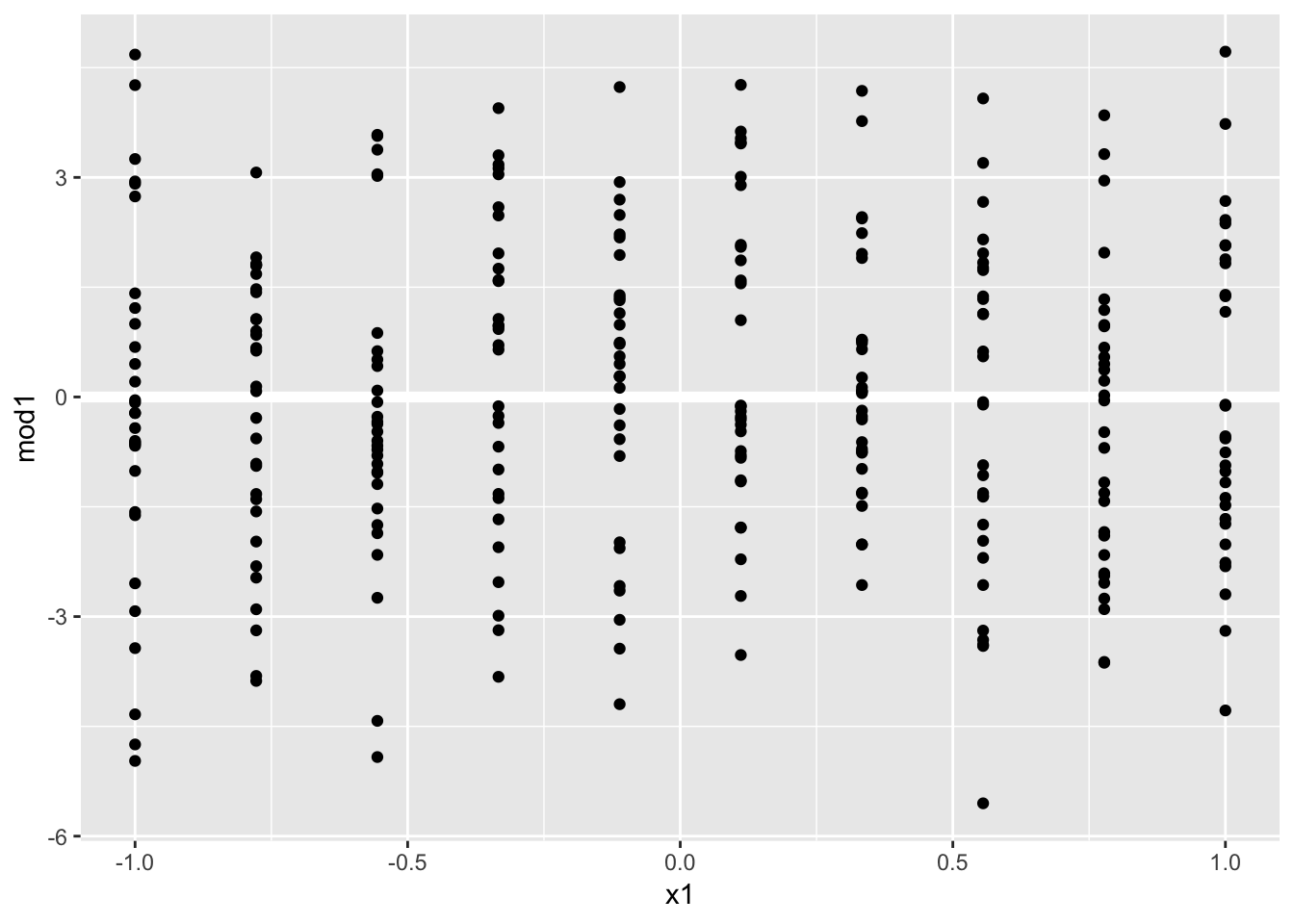
ggplot(sim4, aes(x1, mod2)) +
  geom_ref_line(h = 0) +
geom_point() 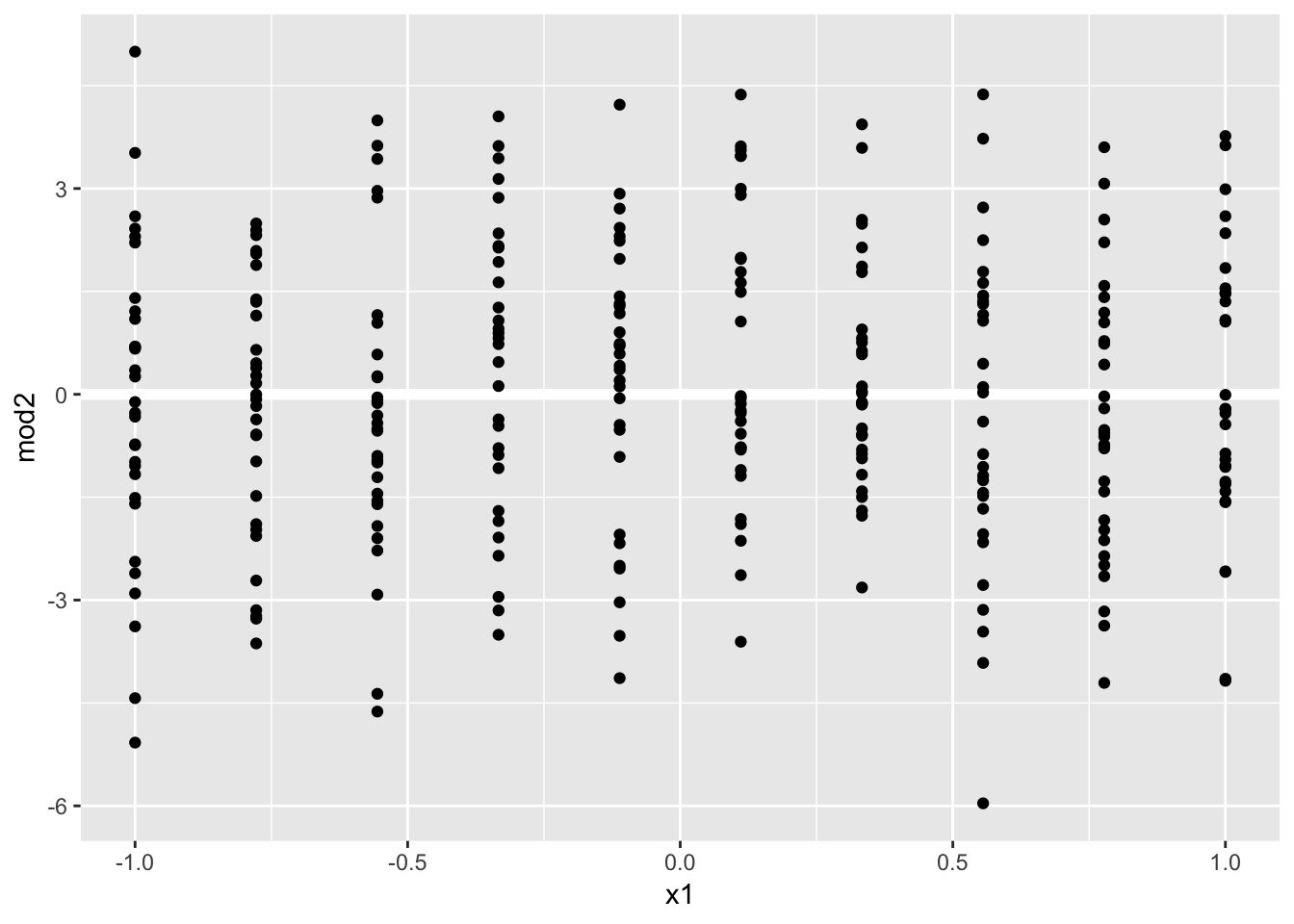
sim4 %>% summarize ( mod1_rmse = sqrt(mean(mod1^2)),
                     mod2_rmse = sqrt(mean(mod2^2)))
## # A tibble: 1 x 2
## mod1_rmse mod2_rmse
## <dbl> <dbl>
## 1 2.10 2.06